yolo类检测算法解析——yolo v3 - greathuman - 博客园

mikel阅读(646)

来源: yolo类检测算法解析——yolo v3 – greathuman – 博客园

每当听到有人问“如何入门计算机视觉”这个问题时,其实我内心是拒绝的,为什么呢?因为我们说的计算机视觉的发展史可谓很长了,它的分支很多,而且理论那是错综复杂交相辉映,就好像数学一样,如何学习数学?这问题似乎有点笼统、有点宽泛。所以我都会具体问问你想入门计算机视觉的哪个话题,只有顺着一个话题理论联合实际,才有可能扩展到几个话题。

yolo类算法,从开始到现在已经有了3代,我们称之为v1、v2、v3,一路走来,让人能感觉到的是算法的性能在不断的改进,以至于现在成为了开源通用目标检测算法的领头羊(ps:虽然本人一直都很欣赏SSD,但是不得不说V3版本已经达到目前的颠覆)。一直以来,有一个问题困扰许久,那就是如何检测两个距离很近的同类的物体,当然又或者是距离很近的不同类的物体?绝大部分算法都会对传入的data做resize到一个更小的resolution,它们对于这种情况都会给出一个目标框,因为在它们的特征提取或者回归过程看来,这就是一个物体(可想本来就很近,一放缩之间的近距离越发明显了),而事实上这是两个同(或不同)类型的物体靠的很近,这个难题是目标检测和跟踪领域的一个挑战。就好像对小目标的检测,一直以来也被看做是算法的一种评估。但是啊,v3版本却做到了,它对这种距离很近的物体或者小物体有很好的鲁棒性,虽然不能保证百分百,但是这个难题得到了很大程度的解决,激发我对yolo类算法的研究。这也是为什么写这篇文章的目的,在于见证一下这个算法的神奇。其实,百分百的检测,在我看来事实上是不存在的,随着时间的推移,环境的变化,任何妄言百分百准确的算法都是扯,只能是相互调整吧。前几天uber撞人事件其实我最关注的应该是哪个环节存在的问题,还需要改进,撞人是不可避免的,无人车的存在不是让事故不发生,而是让社会进步,科技发展,逐步降低事故发生率的同时改善人们的生活质量。

yolo的v1和v2都不如SSD算法,原谅这么直白,原因是v1版本的448和v2版本的416都不如SSD的300,当然以上结论都是实验测的,v3版本的416应该比SSD512好,可见其性能。

对官方yolo做了实验,实验中,采用同一个视频、同一张显卡,在阈值为0.3的前提下,对比了v3和v2的测试效果之后,有了下面两个疑问:

1.为什么v3和v2版本的测试性能提高很大,但速度却没有降低?

2.为什么v3性能上能有这么大的改进?或者说为什么v3在没有提高输入数据分辨率的前提下,对小目标检测变得这么好?

要回答上述两个问题,必须要看看作者发布的v3论文了,将v3和v2不一样的地方总结一下:

  • loss不同:作者v3替换了v2的softmax loss 变成logistic loss,而且每个ground truth只匹配一个先验框。
  • anchor bbox prior不同:v2作者用了5个anchor,一个折衷的选择,所以v3用了9个anchor,提高了IOU。
  • detection的策略不同:v2只有一个detection,v3一下变成了3个,分别是一个下采样的,feature map为13*13,还有2个上采样的eltwise sum,feature map为26*26,52*52,也就是说v3的416版本已经用到了52的feature map,而v2把多尺度考虑到训练的data采样上,最后也只是用到了13的feature map,这应该是对小目标影响最大的地方。
  • backbone不同:这和上一点是有关系的,v2的darknet-19变成了v3的darknet-53,为啥呢?就是需要上采样啊,卷积层的数量自然就多了,另外作者还是用了一连串的3*3、1*1卷积,3*3的卷积增加channel,而1*1的卷积在于压缩3*3卷积后的特征表示,这波操作很具有实用性,一增一减,效果棒棒。

为什么有这么大的提高?我指的是v2和v3比,同样是416的feature map,我感觉是v2作者当时也是做了很多尝试和借鉴,实现了匹敌SSD的效果,但是他因为被借鉴的内容所困扰,导致性能的停留,因此v3再借鉴,应该是参考了DSSD和FPN,这应该是之后的潮流了,做了一下结果性能提高很大,可能作者本人都没想到。但是作者目前没有写篇论文,认为没有创造性实质性的改变,写了一个report,科研的精神值得肯定!如果对比v2和v3你会发现反差确实很大,所以上面的问题才不奇怪。

又为什么速度没有下降?电脑上同环境测都是15帧左右。先看一下打印的日志:

 v2的日志信息:

复制代码
Demo
layer     filters    size              input                output
    0 conv     32  3 x 3 / 1   416 x 416 x   3   ->   416 x 416 x  32  0.299 BFLOPs
    1 max          2 x 2 / 2   416 x 416 x  32   ->   208 x 208 x  32
    2 conv     64  3 x 3 / 1   208 x 208 x  32   ->   208 x 208 x  64  1.595 BFLOPs
    3 max          2 x 2 / 2   208 x 208 x  64   ->   104 x 104 x  64
    4 conv    128  3 x 3 / 1   104 x 104 x  64   ->   104 x 104 x 128  1.595 BFLOPs
    5 conv     64  1 x 1 / 1   104 x 104 x 128   ->   104 x 104 x  64  0.177 BFLOPs
    6 conv    128  3 x 3 / 1   104 x 104 x  64   ->   104 x 104 x 128  1.595 BFLOPs
    7 max          2 x 2 / 2   104 x 104 x 128   ->    52 x  52 x 128
    8 conv    256  3 x 3 / 1    52 x  52 x 128   ->    52 x  52 x 256  1.595 BFLOPs
    9 conv    128  1 x 1 / 1    52 x  52 x 256   ->    52 x  52 x 128  0.177 BFLOPs
   10 conv    256  3 x 3 / 1    52 x  52 x 128   ->    52 x  52 x 256  1.595 BFLOPs
   11 max          2 x 2 / 2    52 x  52 x 256   ->    26 x  26 x 256
   12 conv    512  3 x 3 / 1    26 x  26 x 256   ->    26 x  26 x 512  1.595 BFLOPs
   13 conv    256  1 x 1 / 1    26 x  26 x 512   ->    26 x  26 x 256  0.177 BFLOPs
   14 conv    512  3 x 3 / 1    26 x  26 x 256   ->    26 x  26 x 512  1.595 BFLOPs
   15 conv    256  1 x 1 / 1    26 x  26 x 512   ->    26 x  26 x 256  0.177 BFLOPs
   16 conv    512  3 x 3 / 1    26 x  26 x 256   ->    26 x  26 x 512  1.595 BFLOPs
   17 max          2 x 2 / 2    26 x  26 x 512   ->    13 x  13 x 512
   18 conv   1024  3 x 3 / 1    13 x  13 x 512   ->    13 x  13 x1024  1.595 BFLOPs
   19 conv    512  1 x 1 / 1    13 x  13 x1024   ->    13 x  13 x 512  0.177 BFLOPs
   20 conv   1024  3 x 3 / 1    13 x  13 x 512   ->    13 x  13 x1024  1.595 BFLOPs
   21 conv    512  1 x 1 / 1    13 x  13 x1024   ->    13 x  13 x 512  0.177 BFLOPs
   22 conv   1024  3 x 3 / 1    13 x  13 x 512   ->    13 x  13 x1024  1.595 BFLOPs
   23 conv   1024  3 x 3 / 1    13 x  13 x1024   ->    13 x  13 x1024  3.190 BFLOPs
   24 conv   1024  3 x 3 / 1    13 x  13 x1024   ->    13 x  13 x1024  3.190 BFLOPs
   25 route  16
   26 conv     64  1 x 1 / 1    26 x  26 x 512   ->    26 x  26 x  64  0.044 BFLOPs
   27 reorg              / 2    26 x  26 x  64   ->    13 x  13 x 256
   28 route  27 24
   29 conv   1024  3 x 3 / 1    13 x  13 x1280   ->    13 x  13 x1024  3.987 BFLOPs
   30 conv    125  1 x 1 / 1    13 x  13 x1024   ->    13 x  13 x 125  0.043 BFLOPs
   31 detection
mask_scale: Using default '1.000000'
Loading weights from yolo-voc.weights...Done!
复制代码

v3的日志信息:

复制代码
Demo
layer     filters    size              input                output
    0 conv     32  3 x 3 / 1   416 x 416 x   3   ->   416 x 416 x  32  0.299 BFLOPs
    1 conv     64  3 x 3 / 2   416 x 416 x  32   ->   208 x 208 x  64  1.595 BFLOPs
    2 conv     32  1 x 1 / 1   208 x 208 x  64   ->   208 x 208 x  32  0.177 BFLOPs
    3 conv     64  3 x 3 / 1   208 x 208 x  32   ->   208 x 208 x  64  1.595 BFLOPs
    4 res    1                 208 x 208 x  64   ->   208 x 208 x  64
    5 conv    128  3 x 3 / 2   208 x 208 x  64   ->   104 x 104 x 128  1.595 BFLOPs
    6 conv     64  1 x 1 / 1   104 x 104 x 128   ->   104 x 104 x  64  0.177 BFLOPs
    7 conv    128  3 x 3 / 1   104 x 104 x  64   ->   104 x 104 x 128  1.595 BFLOPs
    8 res    5                 104 x 104 x 128   ->   104 x 104 x 128
    9 conv     64  1 x 1 / 1   104 x 104 x 128   ->   104 x 104 x  64  0.177 BFLOPs
   10 conv    128  3 x 3 / 1   104 x 104 x  64   ->   104 x 104 x 128  1.595 BFLOPs
   11 res    8                 104 x 104 x 128   ->   104 x 104 x 128
   12 conv    256  3 x 3 / 2   104 x 104 x 128   ->    52 x  52 x 256  1.595 BFLOPs
   13 conv    128  1 x 1 / 1    52 x  52 x 256   ->    52 x  52 x 128  0.177 BFLOPs
   14 conv    256  3 x 3 / 1    52 x  52 x 128   ->    52 x  52 x 256  1.595 BFLOPs
   15 res   12                  52 x  52 x 256   ->    52 x  52 x 256
   16 conv    128  1 x 1 / 1    52 x  52 x 256   ->    52 x  52 x 128  0.177 BFLOPs
   17 conv    256  3 x 3 / 1    52 x  52 x 128   ->    52 x  52 x 256  1.595 BFLOPs
   18 res   15                  52 x  52 x 256   ->    52 x  52 x 256
   19 conv    128  1 x 1 / 1    52 x  52 x 256   ->    52 x  52 x 128  0.177 BFLOPs
   20 conv    256  3 x 3 / 1    52 x  52 x 128   ->    52 x  52 x 256  1.595 BFLOPs
   21 res   18                  52 x  52 x 256   ->    52 x  52 x 256
   22 conv    128  1 x 1 / 1    52 x  52 x 256   ->    52 x  52 x 128  0.177 BFLOPs
   23 conv    256  3 x 3 / 1    52 x  52 x 128   ->    52 x  52 x 256  1.595 BFLOPs
   24 res   21                  52 x  52 x 256   ->    52 x  52 x 256
   25 conv    128  1 x 1 / 1    52 x  52 x 256   ->    52 x  52 x 128  0.177 BFLOPs
   26 conv    256  3 x 3 / 1    52 x  52 x 128   ->    52 x  52 x 256  1.595 BFLOPs
   27 res   24                  52 x  52 x 256   ->    52 x  52 x 256
   28 conv    128  1 x 1 / 1    52 x  52 x 256   ->    52 x  52 x 128  0.177 BFLOPs
   29 conv    256  3 x 3 / 1    52 x  52 x 128   ->    52 x  52 x 256  1.595 BFLOPs
   30 res   27                  52 x  52 x 256   ->    52 x  52 x 256
   31 conv    128  1 x 1 / 1    52 x  52 x 256   ->    52 x  52 x 128  0.177 BFLOPs
   32 conv    256  3 x 3 / 1    52 x  52 x 128   ->    52 x  52 x 256  1.595 BFLOPs
   33 res   30                  52 x  52 x 256   ->    52 x  52 x 256
   34 conv    128  1 x 1 / 1    52 x  52 x 256   ->    52 x  52 x 128  0.177 BFLOPs
   35 conv    256  3 x 3 / 1    52 x  52 x 128   ->    52 x  52 x 256  1.595 BFLOPs
   36 res   33                  52 x  52 x 256   ->    52 x  52 x 256
   37 conv    512  3 x 3 / 2    52 x  52 x 256   ->    26 x  26 x 512  1.595 BFLOPs
   38 conv    256  1 x 1 / 1    26 x  26 x 512   ->    26 x  26 x 256  0.177 BFLOPs
   39 conv    512  3 x 3 / 1    26 x  26 x 256   ->    26 x  26 x 512  1.595 BFLOPs
   40 res   37                  26 x  26 x 512   ->    26 x  26 x 512
   41 conv    256  1 x 1 / 1    26 x  26 x 512   ->    26 x  26 x 256  0.177 BFLOPs
   42 conv    512  3 x 3 / 1    26 x  26 x 256   ->    26 x  26 x 512  1.595 BFLOPs
   43 res   40                  26 x  26 x 512   ->    26 x  26 x 512
   44 conv    256  1 x 1 / 1    26 x  26 x 512   ->    26 x  26 x 256  0.177 BFLOPs
   45 conv    512  3 x 3 / 1    26 x  26 x 256   ->    26 x  26 x 512  1.595 BFLOPs
   46 res   43                  26 x  26 x 512   ->    26 x  26 x 512
   47 conv    256  1 x 1 / 1    26 x  26 x 512   ->    26 x  26 x 256  0.177 BFLOPs
   48 conv    512  3 x 3 / 1    26 x  26 x 256   ->    26 x  26 x 512  1.595 BFLOPs
   49 res   46                  26 x  26 x 512   ->    26 x  26 x 512
   50 conv    256  1 x 1 / 1    26 x  26 x 512   ->    26 x  26 x 256  0.177 BFLOPs
   51 conv    512  3 x 3 / 1    26 x  26 x 256   ->    26 x  26 x 512  1.595 BFLOPs
   52 res   49                  26 x  26 x 512   ->    26 x  26 x 512
   53 conv    256  1 x 1 / 1    26 x  26 x 512   ->    26 x  26 x 256  0.177 BFLOPs
   54 conv    512  3 x 3 / 1    26 x  26 x 256   ->    26 x  26 x 512  1.595 BFLOPs
   55 res   52                  26 x  26 x 512   ->    26 x  26 x 512
   56 conv    256  1 x 1 / 1    26 x  26 x 512   ->    26 x  26 x 256  0.177 BFLOPs
   57 conv    512  3 x 3 / 1    26 x  26 x 256   ->    26 x  26 x 512  1.595 BFLOPs
   58 res   55                  26 x  26 x 512   ->    26 x  26 x 512
   59 conv    256  1 x 1 / 1    26 x  26 x 512   ->    26 x  26 x 256  0.177 BFLOPs
   60 conv    512  3 x 3 / 1    26 x  26 x 256   ->    26 x  26 x 512  1.595 BFLOPs
   61 res   58                  26 x  26 x 512   ->    26 x  26 x 512
   62 conv   1024  3 x 3 / 2    26 x  26 x 512   ->    13 x  13 x1024  1.595 BFLOPs
   63 conv    512  1 x 1 / 1    13 x  13 x1024   ->    13 x  13 x 512  0.177 BFLOPs
   64 conv   1024  3 x 3 / 1    13 x  13 x 512   ->    13 x  13 x1024  1.595 BFLOPs
   65 res   62                  13 x  13 x1024   ->    13 x  13 x1024
   66 conv    512  1 x 1 / 1    13 x  13 x1024   ->    13 x  13 x 512  0.177 BFLOPs
   67 conv   1024  3 x 3 / 1    13 x  13 x 512   ->    13 x  13 x1024  1.595 BFLOPs
   68 res   65                  13 x  13 x1024   ->    13 x  13 x1024
   69 conv    512  1 x 1 / 1    13 x  13 x1024   ->    13 x  13 x 512  0.177 BFLOPs
   70 conv   1024  3 x 3 / 1    13 x  13 x 512   ->    13 x  13 x1024  1.595 BFLOPs
   71 res   68                  13 x  13 x1024   ->    13 x  13 x1024
   72 conv    512  1 x 1 / 1    13 x  13 x1024   ->    13 x  13 x 512  0.177 BFLOPs
   73 conv   1024  3 x 3 / 1    13 x  13 x 512   ->    13 x  13 x1024  1.595 BFLOPs
   74 res   71                  13 x  13 x1024   ->    13 x  13 x1024
   75 conv    512  1 x 1 / 1    13 x  13 x1024   ->    13 x  13 x 512  0.177 BFLOPs
   76 conv   1024  3 x 3 / 1    13 x  13 x 512   ->    13 x  13 x1024  1.595 BFLOPs
   77 conv    512  1 x 1 / 1    13 x  13 x1024   ->    13 x  13 x 512  0.177 BFLOPs
   78 conv   1024  3 x 3 / 1    13 x  13 x 512   ->    13 x  13 x1024  1.595 BFLOPs
   79 conv    512  1 x 1 / 1    13 x  13 x1024   ->    13 x  13 x 512  0.177 BFLOPs
   80 conv   1024  3 x 3 / 1    13 x  13 x 512   ->    13 x  13 x1024  1.595 BFLOPs
   81 conv    255  1 x 1 / 1    13 x  13 x1024   ->    13 x  13 x 255  0.088 BFLOPs
   82 detection
   83 route  79
   84 conv    256  1 x 1 / 1    13 x  13 x 512   ->    13 x  13 x 256  0.044 BFLOPs
   85 upsample            2x    13 x  13 x 256   ->    26 x  26 x 256
   86 route  85 61
   87 conv    256  1 x 1 / 1    26 x  26 x 768   ->    26 x  26 x 256  0.266 BFLOPs
   88 conv    512  3 x 3 / 1    26 x  26 x 256   ->    26 x  26 x 512  1.595 BFLOPs
   89 conv    256  1 x 1 / 1    26 x  26 x 512   ->    26 x  26 x 256  0.177 BFLOPs
   90 conv    512  3 x 3 / 1    26 x  26 x 256   ->    26 x  26 x 512  1.595 BFLOPs
   91 conv    256  1 x 1 / 1    26 x  26 x 512   ->    26 x  26 x 256  0.177 BFLOPs
   92 conv    512  3 x 3 / 1    26 x  26 x 256   ->    26 x  26 x 512  1.595 BFLOPs
   93 conv    255  1 x 1 / 1    26 x  26 x 512   ->    26 x  26 x 255  0.177 BFLOPs
   94 detection
   95 route  91
   96 conv    128  1 x 1 / 1    26 x  26 x 256   ->    26 x  26 x 128  0.044 BFLOPs
   97 upsample            2x    26 x  26 x 128   ->    52 x  52 x 128
   98 route  97 36
   99 conv    128  1 x 1 / 1    52 x  52 x 384   ->    52 x  52 x 128  0.266 BFLOPs
  100 conv    256  3 x 3 / 1    52 x  52 x 128   ->    52 x  52 x 256  1.595 BFLOPs
  101 conv    128  1 x 1 / 1    52 x  52 x 256   ->    52 x  52 x 128  0.177 BFLOPs
  102 conv    256  3 x 3 / 1    52 x  52 x 128   ->    52 x  52 x 256  1.595 BFLOPs
  103 conv    128  1 x 1 / 1    52 x  52 x 256   ->    52 x  52 x 128  0.177 BFLOPs
  104 conv    256  3 x 3 / 1    52 x  52 x 128   ->    52 x  52 x 256  1.595 BFLOPs
  105 conv    255  1 x 1 / 1    52 x  52 x 256   ->    52 x  52 x 255  0.353 BFLOPs
  106 detection
Loading weights from yolov3.weights...Done!
复制代码
百度百科:FLOPS(即“每秒浮点运算次数”,“每秒峰值速度”),是“每秒所执行的浮点运算次数”(floating-point operations per second)的缩写。它常被用来估算电脑的执行效能,尤其是在使用到大量浮点运算的科学计算领域中。正因为FLOPS字尾的那个S,代表秒,而不是复数,所以不能省略掉。
在这里所谓的“浮点运算”,实际上包括了所有涉及小数的运算。这类运算在某类应用软件中常常出现,而它们也比整数运算更花时间。现今大部分的处理器中,都有一个专门用来处理浮点运算的“浮点运算器”(FPU)。也因此FLOPS所量测的,实际上就是FPU的执行速度。而最常用来测量FLOPS的基准程式(benchmark)之一,就是Linpack
可能的原因:yolov2是一个纵向自上而下的网络架构,随着channel数目的不断增加,FLOPS是不断增加的,而v3网络架构是横纵交叉的,看着卷积层多,其实很多多channel的卷积层没有继承性,另外,虽然yolov3增加了anchor centroid,但是对ground truth的估计变得更加简单,每个ground truth只匹配一个先验框,而且每个尺度只预测3个框,v2预测5个框。这样的话也降低了复杂度。

所以这发展的历程应该是这样的:

yolo——SSD——yolov2——FPN、Focal loss、DSSD……——yolov3

最后总结,yolo算法的性能一直都没有被v2发挥出来,而真正被v3发挥出来了,v3这次的借鉴效果实在是太好了。

欢迎加入QQ交流群864933024

YOLO-V4源码详解 - 爱旅行的球迷Engineer - 博客园

mikel阅读(622)

来源: YOLO-V4源码详解 – 爱旅行的球迷Engineer – 博客园

一. 整体架构

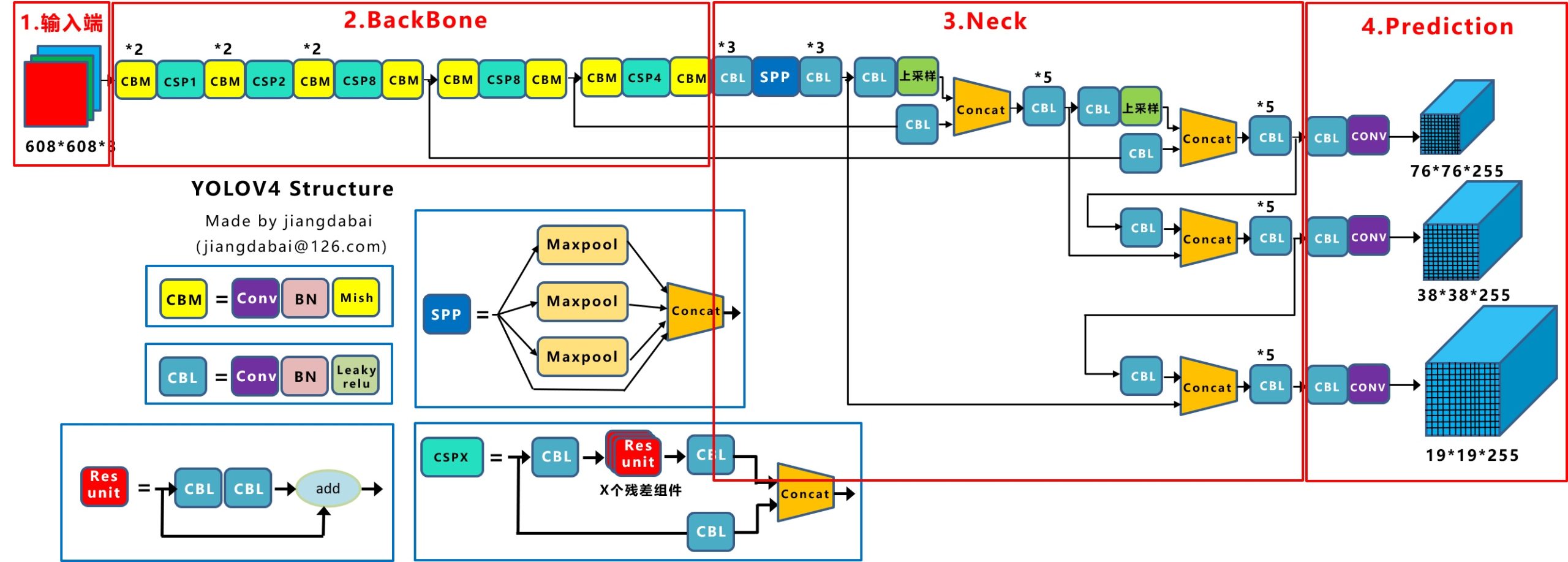
整体架构和YOLO-V3相同(感谢知乎大神@江大白),创新点如下:

输入端 –> Mosaic数据增强、cmBN、SAT自对抗训练;

BackBone –> CSPDarknet53、Mish激活函数、Dropblock;

Neck –> SPP、FPN+PAN结构;

Prediction –> GIOU_Loss、DIOU_nms。

二. 输入端

1. 数据加载流程(以训练为例)

“darknet/src/darknet.c”–main()函数:模型入口。

复制代码
......
    // 根据指令进入不同的函数。
    if (0 == strcmp(argv[1], "average")){
        average(argc, argv);
    } else if (0 == strcmp(argv[1], "yolo")){
        run_yolo(argc, argv);
    } else if (0 == strcmp(argv[1], "voxel")){
        run_voxel(argc, argv);
    } else if (0 == strcmp(argv[1], "super")){
        run_super(argc, argv);
    } else if (0 == strcmp(argv[1], "detector")){
        run_detector(argc, argv); // detector.c中,run_detector函数入口,detect操作,包括训练、测试等。
    } else if (0 == strcmp(argv[1], "detect")){
        float thresh = find_float_arg(argc, argv, "-thresh", .24);
        int ext_output = find_arg(argc, argv, "-ext_output");
        char *filename = (argc > 4) ? argv[4]: 0;
        test_detector("cfg/coco.data", argv[2], argv[3], filename, thresh, 0.5, 0, ext_output, 0, NULL, 0, 0);
......
复制代码

“darknet/src/detector.c”–run_detector()函数:train指令入口。

复制代码
......
    if (0 == strcmp(argv[2], "test")) test_detector(datacfg, cfg, weights, filename, thresh, hier_thresh, dont_show, ext_output, save_labels, outfile, letter_box, benchmark_layers); // 测试test_detector函数入口。
    else if (0 == strcmp(argv[2], "train")) train_detector(datacfg, cfg, weights, gpus, ngpus, clear, dont_show, calc_map, mjpeg_port, show_imgs, benchmark_layers, chart_path); // 训练train_detector函数入口。
    else if (0 == strcmp(argv[2], "valid")) validate_detector(datacfg, cfg, weights, outfile);
......
复制代码

“darknet/src/detector.c”–train_detector()函数:数据加载入口。

pthread_t load_thread = load_data(args); // 首次创建并启动加载线程,args为模型训练参数。

“darknet/src/data.c”–load_data()函数:load_threads()分配线程。

复制代码
pthread_t load_data(load_args args) 
{
    pthread_t thread;
    struct load_args* ptr = (load_args*)xcalloc(1, sizeof(struct load_args));
    *ptr = args;
    /* 调用load_threads()函数。 */
    if(pthread_create(&thread, 0, load_threads, ptr)) error("Thread creation failed"); // 参数1:指向线程标识符的指针;参数2:设置线程属性;参数3:线程运行函数的地址;参数4:运行函数的参数。
    return thread;
}
复制代码

“darknet/src/data.c”–load_threads()函数中:多线程调用run_thread_loop()。

复制代码
if (!threads) {
    threads = (pthread_t*)xcalloc(args.threads, sizeof(pthread_t));
    run_load_data = (volatile int *)xcalloc(args.threads, sizeof(int));
    args_swap = (load_args *)xcalloc(args.threads, sizeof(load_args));
    fprintf(stderr, " Create %d permanent cpu-threads \n", args.threads);
    for (i = 0; i < args.threads; ++i) {
        int* ptr = (int*)xcalloc(1, sizeof(int));
        *ptr = i;
        if (pthread_create(&threads[i], 0, run_thread_loop, ptr)) error("Thread creation failed"); // 根据线程个数,调用run_thread_loop函数。
    }
}
复制代码

“darknet/src/data.c”–run_thread_loop函数:根据线程ID调用load_thread()。

复制代码
void *run_thread_loop(void *ptr)
{
    const int i = *(int *)ptr;
    while (!custom_atomic_load_int(&flag_exit)) {
        while (!custom_atomic_load_int(&run_load_data[i])) {
            if (custom_atomic_load_int(&flag_exit)) {
                free(ptr);
                return 0;
            }
            this_thread_sleep_for(thread_wait_ms);
        }
        pthread_mutex_lock(&mtx_load_data);
        load_args *args_local = (load_args *)xcalloc(1, sizeof(load_args));
        *args_local = args_swap[i]; // 传入线程ID,在load_threads()函数中args_swap[i] = args。
        pthread_mutex_unlock(&mtx_load_data);
        load_thread(args_local); // 调用load_thread()函数。
        custom_atomic_store_int(&run_load_data[i], 0);
    }
    free(ptr);
    return 0;
}
复制代码

“darknet/src/data.c”–load_thread()函数中:根据type标识符执行最底层的数据加载任务load_data_detection()。

else if (a.type == DETECTION_DATA){ // 用于检测的数据,在train_detector()函数中,args.type = DETECTION_DATA。
        *a.d = load_data_detection(a.n, a.paths, a.m, a.w, a.h, a.c, a.num_boxes, a.classes, a.flip, a.gaussian_noise, a.blur, a.mixup, a.jitter, a.resize,
            a.hue, a.saturation, a.exposure, a.mini_batch, a.track, a.augment_speed, a.letter_box, a.show_imgs);

“darknet/src/data.c”–load_data_detection()函数根据是否配置opencv,有两个版本,opencv版本中:

基本数据处理:

包括crop、flip、HSV augmentation、blur以及gaussian_noise。(注意,a.type == DETECTION_DATA时,无angle参数传入,没有图像旋转增强)

复制代码
......
        if (track) random_paths = get_sequential_paths(paths, n, m, mini_batch, augment_speed); // 目标跟踪。
        else random_paths = get_random_paths(paths, n, m); // 随机选取n张图片的路径。
        for (i = 0; i < n; ++i) {
            float *truth = (float*)xcalloc(5 * boxes, sizeof(float));
            const char *filename = random_paths[i];
            int flag = (c >= 3);
            mat_cv *src;
            src = load_image_mat_cv(filename, flag); // image_opencv.cpp中,load_image_mat_cv函数入口,使用opencv读取图像。
......
            /* 将原图进行一定比例的缩放。 */
            if (letter_box) 
            {
                float img_ar = (float)ow / (float)oh; // 读取到的原始图像宽高比。
                float net_ar = (float)w / (float)h; // 规定的,输入到网络要求的图像宽高比。
                float result_ar = img_ar / net_ar; // 两者求比值来判断如何进行letter_box缩放。
                if (result_ar > 1)  // sheight - should be increased
                {
                    float oh_tmp = ow / net_ar;
                    float delta_h = (oh_tmp - oh)/2;
                    ptop = ptop - delta_h;
                    pbot = pbot - delta_h;
                }
                else  // swidth - should be increased
                {
                    float ow_tmp = oh * net_ar;
                    float delta_w = (ow_tmp - ow)/2;
                    pleft = pleft - delta_w;
                    pright = pright - delta_w;
                }
            }
            /* 执行letter_box变换。 */
            int swidth = ow - pleft - pright;
            int sheight = oh - ptop - pbot;
            float sx = (float)swidth / ow;
            float sy = (float)sheight / oh;
            float dx = ((float)pleft / ow) / sx;
            float dy = ((float)ptop / oh) / sy;
            /* truth在调用函数后获得所有图像的标签信息,因为对原始图片进行了数据增强,其中的平移抖动势必会改动每个物体的矩形框标签信息,需要根据具体的数据增强方式进行相应矫正,后面的参数就是用于数据增强后的矩形框信息矫正。 */
            int min_w_h = fill_truth_detection(filename, boxes, truth, classes, flip, dx, dy, 1. / sx, 1. / sy, w, h); // 求最小obj尺寸。
            if ((min_w_h / 8) < blur && blur > 1) blur = min_w_h / 8;   // disable blur if one of the objects is too small
            // image_opencv.cpp中,image_data_augmentation函数入口,数据增强。
            image ai = image_data_augmentation(src, w, h, pleft, ptop, swidth, sheight, flip, dhue, dsat, dexp, gaussian_noise, blur, boxes, truth);
......
复制代码

“darknet/src/image_opencv.cpp”–image_data_augmentation()函数:

复制代码
extern "C" image image_data_augmentation(mat_cv* mat, int w, int h, int pleft, int ptop, int swidth, int sheight, int flip,
    float dhue, float dsat, float dexp, int gaussian_noise, int blur, int num_boxes, float *truth)
{
    image out;
    try {
        cv::Mat img = *(cv::Mat *)mat; // 读取图像数据。
        // crop
        cv::Rect src_rect(pleft, ptop, swidth, sheight);
        cv::Rect img_rect(cv::Point2i(0, 0), img.size());
        cv::Rect new_src_rect = src_rect & img_rect;
        cv::Rect dst_rect(cv::Point2i(std::max<int>(0, -pleft), std::max<int>(0, -ptop)), new_src_rect.size());
        cv::Mat sized;
        if (src_rect.x == 0 && src_rect.y == 0 && src_rect.size() == img.size()) {
            cv::resize(img, sized, cv::Size(w, h), 0, 0, cv::INTER_LINEAR);
        }
        else {
            cv::Mat cropped(src_rect.size(), img.type());
            cropped.setTo(cv::mean(img));
            img(new_src_rect).copyTo(cropped(dst_rect));
            // resize
            cv::resize(cropped, sized, cv::Size(w, h), 0, 0, cv::INTER_LINEAR);
        }
        // flip,虽然配置文件里没有flip参数,但代码里有使用。
        if (flip) {
            cv::Mat cropped;
            cv::flip(sized, cropped, 1); // 0 - x-axis, 1 - y-axis, -1 - both axes (x & y)
            sized = cropped.clone();
        }
        // HSV augmentation
        if (dsat != 1 || dexp != 1 || dhue != 0) {
            if (img.channels() >= 3)
            {
                cv::Mat hsv_src;
                cvtColor(sized, hsv_src, cv::COLOR_RGB2HSV); // RGB to HSV
                std::vector<cv::Mat> hsv;
                cv::split(hsv_src, hsv);
                hsv[1] *= dsat;
                hsv[2] *= dexp;
                hsv[0] += 179 * dhue;
                cv::merge(hsv, hsv_src);
                cvtColor(hsv_src, sized, cv::COLOR_HSV2RGB); // HSV to RGB (the same as previous)
            }
            else
            {
                sized *= dexp;
            }
        }
        if (blur) {
            cv::Mat dst(sized.size(), sized.type());
            if (blur == 1) {
                cv::GaussianBlur(sized, dst, cv::Size(17, 17), 0);
            }
            else {
                int ksize = (blur / 2) * 2 + 1;
                cv::Size kernel_size = cv::Size(ksize, ksize);
                cv::GaussianBlur(sized, dst, kernel_size, 0);
            }
            if (blur == 1) {
                cv::Rect img_rect(0, 0, sized.cols, sized.rows);
                int t;
                for (t = 0; t < num_boxes; ++t) {
                    box b = float_to_box_stride(truth + t*(4 + 1), 1);
                    if (!b.x) break;
                    int left = (b.x - b.w / 2.)*sized.cols;
                    int width = b.w*sized.cols;
                    int top = (b.y - b.h / 2.)*sized.rows;
                    int height = b.h*sized.rows;
                    cv::Rect roi(left, top, width, height);
                    roi = roi & img_rect;
                    sized(roi).copyTo(dst(roi));
                }
            }
            dst.copyTo(sized);
        }
        if (gaussian_noise) {
            cv::Mat noise = cv::Mat(sized.size(), sized.type());
            gaussian_noise = std::min(gaussian_noise, 127);
            gaussian_noise = std::max(gaussian_noise, 0);
            cv::randn(noise, 0, gaussian_noise); //mean and variance
            cv::Mat sized_norm = sized + noise;
            sized = sized_norm;
        }
        // Mat -> image
        out = mat_to_image(sized);
    }
    catch (...) {
        cerr << "OpenCV can't augment image: " << w << " x " << h << " \n";
        out = mat_to_image(*(cv::Mat*)mat);
    }
    return out;
}
复制代码

高级数据处理:

主要是mosaic数据增强。

复制代码
......
            if (use_mixup == 0) { // 不使用mixup。
                d.X.vals[i] = ai.data;
                memcpy(d.y.vals[i], truth, 5 * boxes * sizeof(float)); // C库函数,从存储区truth复制5 * boxes * sizeof(float)个字节到存储区d.y.vals[i]。
            }
            else if (use_mixup == 1) { // 使用mixup。
                if (i_mixup == 0) { // 第一个序列。
                    d.X.vals[i] = ai.data;
                    memcpy(d.y.vals[i], truth, 5 * boxes * sizeof(float)); // n张图的label->d.y.vals,i_mixup=1时,作为上一个sequence的label。
                }
                else if (i_mixup == 1) { // 第二个序列,此时d.X.vals已经储存上个序列n张增强后的图。
                    image old_img = make_empty_image(w, h, c);
                    old_img.data = d.X.vals[i]; // 记录上一个序列的n张old_img。
                    blend_images_cv(ai, 0.5, old_img, 0.5); // image_opencv.cpp中,blend_images_cv函数入口,新旧序列对应的两张图进行线性融合,ai只是在i_mixup和i循环最里层的一张图。
                    blend_truth(d.y.vals[i], boxes, truth); // 上一个序列的d.y.vals[i]与这个序列的truth融合。
                    free_image(old_img); // 释放img数据。
                    d.X.vals[i] = ai.data; // 保存这个序列的n张图。
                }
            }
            else if (use_mixup == 3) { // mosaic数据增强。
                if (i_mixup == 0) { // 第一序列,初始化。
                    image tmp_img = make_image(w, h, c);
                    d.X.vals[i] = tmp_img.data;
                }
                if (flip) { // 翻转。
                    int tmp = pleft;
                    pleft = pright;
                    pright = tmp;
                }
                const int left_shift = min_val_cmp(cut_x[i], max_val_cmp(0, (-pleft*w / ow))); // utils.h中,min_val_cmp函数入口,取小(min)取大(max)。
                const int top_shift = min_val_cmp(cut_y[i], max_val_cmp(0, (-ptop*h / oh))); // ptop<0时,取cut_y[i]与-ptop*h / oh较小的,否则返回0。
                const int right_shift = min_val_cmp((w - cut_x[i]), max_val_cmp(0, (-pright*w / ow)));
                const int bot_shift = min_val_cmp(h - cut_y[i], max_val_cmp(0, (-pbot*h / oh)));
                int k, x, y;
                for (k = 0; k < c; ++k) { // 通道。
                    for (y = 0; y < h; ++y) { // 高度。
                        int j = y*w + k*w*h; // 每张图i,按行堆叠索引j。
                        if (i_mixup == 0 && y < cut_y[i]) { // 右下角区块,i_mixup=0~3,d.X.vals[i]未被清0,累计粘贴4块区域。
                            int j_src = (w - cut_x[i] - right_shift) + (y + h - cut_y[i] - bot_shift)*w + k*w*h;
                            memcpy(&d.X.vals[i][j + 0], &ai.data[j_src], cut_x[i] * sizeof(float)); // 由ai.data[j_src]所指内存区域复制cut_x[i]*sizeof(float)个字节到&d.X.vals[i][j + 0]所指内存区域。
                        }
                        if (i_mixup == 1 && y < cut_y[i]) { // 左下角区块。
                            int j_src = left_shift + (y + h - cut_y[i] - bot_shift)*w + k*w*h;
                            memcpy(&d.X.vals[i][j + cut_x[i]], &ai.data[j_src], (w-cut_x[i]) * sizeof(float));
                        }
                        if (i_mixup == 2 && y >= cut_y[i]) { // 右上角区块。
                            int j_src = (w - cut_x[i] - right_shift) + (top_shift + y - cut_y[i])*w + k*w*h;
                            memcpy(&d.X.vals[i][j + 0], &ai.data[j_src], cut_x[i] * sizeof(float));
                        }
                        if (i_mixup == 3 && y >= cut_y[i]) { // 左上角区块。
                            int j_src = left_shift + (top_shift + y - cut_y[i])*w + k*w*h;
                            memcpy(&d.X.vals[i][j + cut_x[i]], &ai.data[j_src], (w - cut_x[i]) * sizeof(float));
                        }
                    }
                }
                blend_truth_mosaic(d.y.vals[i], boxes, truth, w, h, cut_x[i], cut_y[i], i_mixup, left_shift, right_shift, top_shift, bot_shift); // label对应shift调整。
                free_image(ai);
                ai.data = d.X.vals[i];
            }
......
复制代码

三. BackBone

总图:

网络配置文件(.cfg)决定了模型架构,训练时需要在命令行指定。文件以[net]段开头,定义与训练直接相关的参数:

复制代码
[net]
# Testing # 测试时,batch和subdivisions设置为1,否则可能出错。
#batch=1 # 大一些可以减小训练震荡及训练时NAN的出现。
#subdivisions=1 # 必须为为8的倍数,显存吃紧可以设成32或64。
# Training
batch=64 # 训练过程中将64张图一次性加载进内存,前向传播后将64张图的loss累加求平均,再一次性后向传播更新权重。
subdivisions=16 # 一个batch分16次完成前向传播,即每次计算4张。
width=608 # 网络输入的宽。
height=608 # 网络输入的高。
channels=3 # 网络输入的通道数。
momentum=0.949 # 动量梯度下降优化方法中的动量参数,更新的时候在一定程度上保留之前更新的方向。
decay=0.0005 # 权重衰减正则项,用于防止过拟合。
angle=0 # 数据增强参数,通过旋转角度来生成更多训练样本。
saturation = 1.5 # 数据增强参数,通过调整饱和度来生成更多训练样本。
exposure = 1.5 # 数据增强参数,通过调整曝光量来生成更多训练样本。
hue=.1 # 数据增强参数,通过调整色调来生成更多训练样本。
learning_rate=0.001 # 学习率。
burn_in=1000 # 在迭代次数小于burn_in时,学习率的更新为一种方式,大于burn_in时,采用policy的更新方式。
max_batches = 500500 #训练迭代次数,跑完一个batch为一次,一般为类别数*2000,训练样本少或train from scratch可适当增加。
policy=steps # 学习率调整的策略。
steps=400000,450000 # 动态调整学习率,steps可以取max_batches的0.8~0.9。
scales=.1,.1 # 迭代到steps(1)次时,学习率衰减十倍,steps(2)次时,学习率又会在前一个学习率的基础上衰减十倍。
#cutmix=1 # cutmix数据增强,将一部分区域cut掉但不填充0像素而是随机填充训练集中的其他数据的区域像素值,分类结果按一定的比例分配。
mosaic=1 # 马赛克数据增强,取四张图,随机缩放、随机裁剪、随机排布的方式拼接,详见上述代码分析。
复制代码

其余区段,包括[convolutional]、[route]、[shortcut]、[maxpool]、[upsample]、[yolo]层,为不同类型的层的配置参数。YOLO-V4中[net]层之后堆叠多个CBM及CSP层,首先是2个CBM层,CBM结构如下:

复制代码
[convolutional]
batch_normalize=1 # 是否进行BN。
filters=32 # 卷积核个数,也就是该层的输出通道数。
size=3 # 卷积核大小。
stride=1 # 卷积步长。
pad=1 # pad边缘补像素。
activation=mish # 网络层激活函数,yolo-v4只在Backbone中采用了mish,网络后面仍采用Leaky_relu。
复制代码

创新点是Mish激活函数,与Leaky_Relu曲线对比如图:

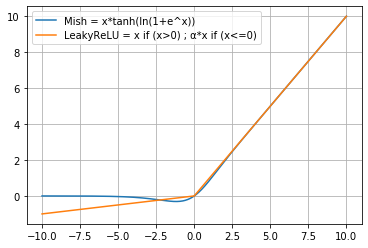
Mish在负值的时候并不是完全截断,而是允许比较小的负梯度流入,保证了信息的流动。此外,平滑的激活函数允许更好的信息深入神经网络,梯度下降效果更好,从而提升准确性和泛化能力。

两个CBM后是CSP1,CSP1结构如下:

复制代码
# CSP1 = CBM + 1个残差unit + CBM -> Concat(with CBM),见总图。
[convolutional] # CBM层,直接与7层后的route层连接,形成总图中CSPX下方支路。
batch_normalize=1
filters=64
size=1
stride=1
pad=1
activation=mish

[route] # 得到前面第2层的输出,即CSP开始位置,构建如图所示的CSP第一支路。
layers = -2

[convolutional] # CBM层。
batch_normalize=1
filters=64
size=1
stride=1
pad=1
activation=mish

# Residual Block
[convolutional] # CBM层。
batch_normalize=1
filters=32
size=1
stride=1
pad=1
activation=mish

[convolutional] # CBM层。
batch_normalize=1
filters=64
size=3
stride=1
pad=1
activation=mish

[shortcut] # add前面第3层的输出,Residual Block结束。
from=-3
activation=linear

[convolutional] # CBM层。
batch_normalize=1
filters=64
size=1
stride=1
pad=1
activation=mish

[route] # Concat上一个CBM层与前面第7层(CBM)的输出。
layers = -1,-7
复制代码

接下来的CBM及CSPX架构与上述block相同,只是CSPX对应X个残差单元,如图:

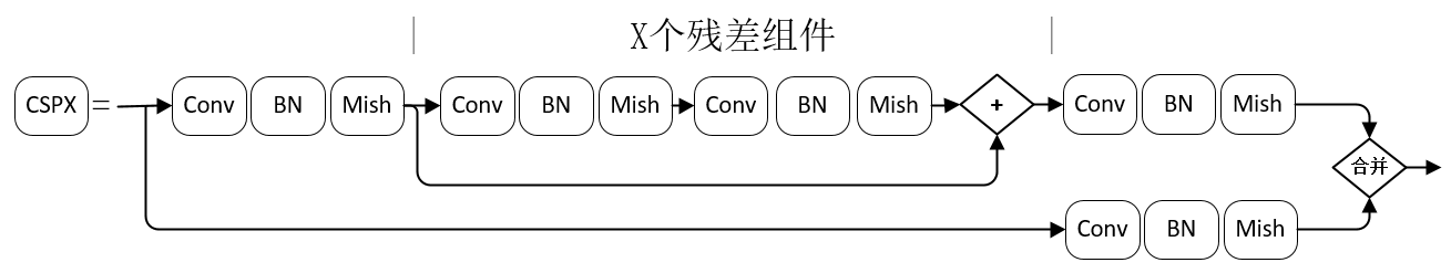
CSP模块将基础层的特征映射划分为两部分,再skip connection,减少计算量的同时保证了准确率。

要注意的是,backbone中两次出现分支,与后续Neck连接,稍后会解释。

四. Neck&Prediction

.cfg配置文件后半部分是Neck和YOLO-Prediction设置,我做了重点注释:

复制代码
### CBL*3 ###
[convolutional]
batch_normalize=1
filters=512
size=1
stride=1
pad=1
activation=leaky # 不再使用Mish。

[convolutional]
batch_normalize=1
size=3
stride=1
pad=1
filters=1024
activation=leaky

[convolutional]
batch_normalize=1
filters=512
size=1
stride=1
pad=1
activation=leaky

### SPP-最大池化的方式进行多尺度融合 ###
[maxpool] # 5*5。
stride=1
size=5

[route]
layers=-2

[maxpool] # 9*9。
stride=1
size=9

[route]
layers=-4

[maxpool] # 13*13。
stride=1
size=13

[route] # Concat。
layers=-1,-3,-5,-6
### End SPP ###

### CBL*3 ###
[convolutional]
batch_normalize=1
filters=512
size=1
stride=1
pad=1
activation=leaky # 不再使用Mish。

[convolutional]
batch_normalize=1
size=3
stride=1
pad=1
filters=1024
activation=leaky

[convolutional]
batch_normalize=1
filters=512
size=1
stride=1
pad=1
activation=leaky

### CBL ###
[convolutional]
batch_normalize=1
filters=256
size=1
stride=1
pad=1
activation=leaky

### 上采样 ###
[upsample]
stride=2

[route]
layers = 85 # 获取Backbone中CBM+CSP8+CBM模块的输出,85从net以外的层开始计数,从0开始索引。

[convolutional] # 增加CBL支路。
batch_normalize=1 
filters=256
size=1
stride=1
pad=1
activation=leaky

[route] # Concat。
layers = -1, -3

### CBL*5 ###
[convolutional]
batch_normalize=1
filters=256
size=1
stride=1
pad=1
activation=leaky

[convolutional]
batch_normalize=1
size=3
stride=1
pad=1
filters=512
activation=leaky

[convolutional]
batch_normalize=1
filters=256
size=1
stride=1
pad=1
activation=leaky

[convolutional]
batch_normalize=1
size=3
stride=1
pad=1
filters=512
activation=leaky

[convolutional]
batch_normalize=1
filters=256
size=1
stride=1
pad=1
activation=leaky

### CBL ###
[convolutional]
batch_normalize=1
filters=128
size=1
stride=1
pad=1
activation=leaky

### 上采样 ###
[upsample]
stride=2

[route]
layers = 54 # 获取Backbone中CBM*2+CSP1+CBM*2+CSP2+CBM*2+CSP8+CBM模块的输出,54从net以外的层开始计数,从0开始索引。

### CBL ###
[convolutional]
batch_normalize=1
filters=128
size=1
stride=1
pad=1
activation=leaky

[route] # Concat。
layers = -1, -3

### CBL*5 ###
[convolutional]
batch_normalize=1
filters=128
size=1
stride=1
pad=1
activation=leaky

[convolutional]
batch_normalize=1
size=3
stride=1
pad=1
filters=256
activation=leaky

[convolutional]
batch_normalize=1
filters=128
size=1
stride=1
pad=1
activation=leaky

[convolutional]
batch_normalize=1
size=3
stride=1
pad=1
filters=256
activation=leaky

[convolutional]
batch_normalize=1
filters=128
size=1
stride=1
pad=1
activation=leaky

### Prediction ###
### CBL ###
[convolutional]
batch_normalize=1
size=3
stride=1
pad=1
filters=256
activation=leaky

### conv ###
[convolutional]
size=1
stride=1
pad=1
filters=255
activation=linear
[yolo] # 76*76*255,对应最小的anchor box。
mask = 0,1,2 # 当前属于第几个预选框。
# coco数据集默认值,可通过detector calc_anchors,利用k-means计算样本anchors,但要根据每个anchor的大小(是否超过60*60或30*30)更改mask对应的索引(第一个yolo层对应小尺寸;第二个对应中等大小;第三个对应大尺寸)及上一个conv层的filters。
anchors = 12, 16, 19, 36, 40, 28, 36, 75, 76, 55, 72, 146, 142, 110, 192, 243, 459, 401
classes=80 # 网络需要识别的物体种类数。
num=9 # 预选框的个数,即anchors总数。
jitter=.3 # 通过抖动增加噪声来抑制过拟合。
ignore_thresh = .7
truth_thresh = 1
scale_x_y = 1.2
iou_thresh=0.213
cls_normalizer=1.0
iou_normalizer=0.07
iou_loss=ciou # CIOU损失函数,考虑目标框回归函数的重叠面积、中心点距离及长宽比。
nms_kind=greedynms
beta_nms=0.6
max_delta=5
[route]
layers = -4 # 获取Neck第一层的输出。

### 构建第二分支 ###
### CBL ###
[convolutional]
batch_normalize=1
size=3
stride=2
pad=1
filters=256
activation=leaky

[route] # Concat。
layers = -1, -16

### CBL*5 ###
[convolutional]
batch_normalize=1
filters=256
size=1
stride=1
pad=1
activation=leaky

[convolutional]
batch_normalize=1
size=3
stride=1
pad=1
filters=512
activation=leaky

[convolutional]
batch_normalize=1
filters=256
size=1
stride=1
pad=1
activation=leaky

[convolutional]
batch_normalize=1
size=3
stride=1
pad=1
filters=512
activation=leaky

[convolutional]
batch_normalize=1
filters=256
size=1
stride=1
pad=1
activation=leaky

### CBL ###
[convolutional]
batch_normalize=1
size=3
stride=1
pad=1
filters=512
activation=leaky

### conv ###
[convolutional]
size=1
stride=1
pad=1
filters=255
activation=linear

[yolo] # 38*38*255,对应中等的anchor box。
mask = 3,4,5
anchors = 12, 16, 19, 36, 40, 28, 36, 75, 76, 55, 72, 146, 142, 110, 192, 243, 459, 401
classes=80
num=9
jitter=.3
ignore_thresh = .7
truth_thresh = 1
scale_x_y = 1.1
iou_thresh=0.213
cls_normalizer=1.0
iou_normalizer=0.07
iou_loss=ciou
nms_kind=greedynms
beta_nms=0.6
max_delta=5

[route] # 获取Neck第二层的输出。
layers = -4

### 构建第三分支 ###
### CBL ###
[convolutional]
batch_normalize=1
size=3
stride=2
pad=1
filters=512
activation=leaky

[route] # Concat。
layers = -1, -37

### CBL*5 ###
[convolutional]
batch_normalize=1
filters=512
size=1
stride=1
pad=1
activation=leaky

[convolutional]
batch_normalize=1
size=3
stride=1
pad=1
filters=1024
activation=leaky

[convolutional]
batch_normalize=1
filters=512
size=1
stride=1
pad=1
activation=leaky

[convolutional]
batch_normalize=1
size=3
stride=1
pad=1
filters=1024
activation=leaky

[convolutional]
batch_normalize=1
filters=512
size=1
stride=1
pad=1
activation=leaky

### CBL ###
[convolutional]
batch_normalize=1
size=3
stride=1
pad=1
filters=1024
activation=leaky

### conv ###
[convolutional]
size=1
stride=1
pad=1
filters=255
activation=linear

[yolo] # 19*19*255,对应最大的anchor box。
mask = 6,7,8
anchors = 12, 16, 19, 36, 40, 28, 36, 75, 76, 55, 72, 146, 142, 110, 192, 243, 459, 401
classes=80
num=9
jitter=.3
ignore_thresh = .7
truth_thresh = 1
random=1
scale_x_y = 1.05
iou_thresh=0.213
cls_normalizer=1.0
iou_normalizer=0.07
iou_loss=ciou
nms_kind=greedynms
beta_nms=0.6
max_delta=5

复制代码

其中第一个创新点是引入Spatial Pyramid Pooling(SPP)模块:

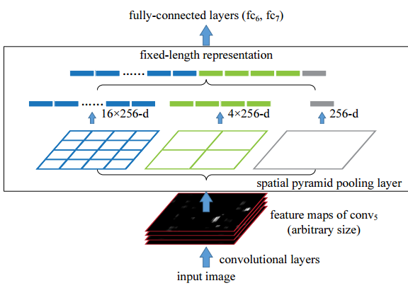
代码中max pool和route层组合,三个不同尺度的max-pooling将前一个卷积层输出的feature maps进行多尺度的特征处理,再与原图进行拼接,一共4个scale。相比于只用一个max-pooling,提取的特征范围更大,而且将不同尺度的特征进行了有效分离;

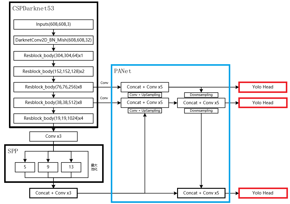
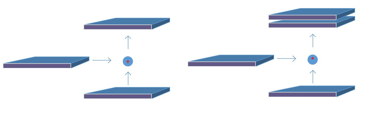
第二个创新点是在FPN的基础上引入PAN结构:

原版PANet中PAN操作是做element-wise相加,YOLO-V4则采用扩增维度的Concat,如下图:

Backbone下采样不同阶段得到的特征图Concat后续上采样阶对应尺度的的output,形成FPN结构,再经过两个botton-up的PAN结构。

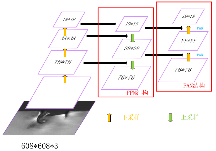
下采样1:前10个block中,只有3个CBM的stride为2,输入图像尺寸变为608/2*2*2=76,filters根据最后一个CBM为256,因此第10个block输出feature map为76*76*256;

下采样2:继续Backbone,同理,第13个block(CBM)输出38*38*512的特征图;

下采样3:第23个block(CBL)输出为19*19*512;

上采样1:下采样3 + CBL + 上采样 = 38*38*256;

Concat1:[上采样1] Concat [下采样2 + CBL] = [38*38*256] Concat [38*38*512 + (256,1)] = 38*38*512;

上采样2:Concat1 + CBL*5 + CBL + 上采样 = 76*76*128;

Concat2:[上采样2] Concat [下采样1 + CBL] = [76*76*128] Concat [76*76*256 + (128,1)] = 76*76*256;

Concat3(PAN1):[Concat2 + CBL*5 + CBL] Concat [Concat1 + CBL*5] = [76*76*256 + (128,1) + (256,2)] Concat [38*38*512 + (256,1)] = [38*38*256] Concat [38*38*256] = 38*38*512;

Concat4(PAN2):[Concat3 + CBL*5 + CBL] Concat [下采样3] = [38*38*512 + (256,1) + (512,2)] Concat [19*19*512] = 19*19*1024;

Prediction①:Concat2 + CBL*5 + CBL + conv = 76*76*256 + (128,1) + (256,1) + (filters,1) = 76*76*filters,其中filters = (class_num + 5)*3,图中默认COCO数据集,80类所以是255;

Prediction②:PAN1 + CBL*5 + CBL + conv = 38*38*512 + (256,1) + (512,1) + (filters,1) = 38*38*filters,其中filters = (class_num + 5)*3,图中默认COCO数据集,80类所以是255;

Prediction③:PAN2 + CBL*5 + CBL + conv = 19*19*1024 + (512,1) + (1024,1) + (filters,1) = 19*19*filters,其中filters = (class_num + 5)*3,图中默认COCO数据集,80类所以是255。

五. 网络构建

上述从backbone到prediction的网络架构,源码中都是基于network结构体来储存网络参数。具体流程如下:

“darknet/src/detector.c”–train_detector()函数中:

复制代码
......    
    network net_map;
    if (calc_map) { // 计算mAP。
        ......
        net_map = parse_network_cfg_custom(cfgfile, 1, 1); // parser.c中parse_network_cfg_custom函数入口,加载cfg和参数构建网络,batch = 1。
        net_map.benchmark_layers = benchmark_layers;
        const int net_classes = net_map.layers[net_map.n - 1].classes;
        int k;  // free memory unnecessary arrays
        for (k = 0; k < net_map.n - 1; ++k) free_layer_custom(net_map.layers[k], 1);
        ......
    }
    srand(time(0));
    char *base = basecfg(cfgfile); // utils.c中basecfg()函数入口,解析cfg/yolo-obj.cfg文件,就是模型的配置参数,并打印。
    printf("%s\n", base);
    float avg_loss = -1;
    network* nets = (network*)xcalloc(ngpus, sizeof(network)); // 给network结构体分内存,用来储存网络参数。
    srand(time(0));
    int seed = rand();
    int k;
    for (k = 0; k < ngpus; ++k) {
        srand(seed);
#ifdef GPU
        cuda_set_device(gpus[k]);
#endif
        nets[k] = parse_network_cfg(cfgfile); // parse_network_cfg_custom(cfgfile, 0, 0),nets根据GPU个数分别加载配置文件。
        nets[k].benchmark_layers = benchmark_layers;
        if (weightfile) {
            load_weights(&nets[k], weightfile); // parser.c中load_weights()接口,读取权重文件。
        }
        if (clear) { // 是否清零。
            *nets[k].seen = 0;
            *nets[k].cur_iteration = 0;
        }
        nets[k].learning_rate *= ngpus;
    }
    srand(time(0));
    network net = nets[0]; // 参数传递给net
    ......
    /* 准备加载参数。 */
    load_args args = { 0 };
    args.w = net.w;
    args.h = net.h;
    args.c = net.c;
    args.paths = paths;
    args.n = imgs;
    args.m = plist->size;
    args.classes = classes;
    args.flip = net.flip;
    args.jitter = l.jitter;
    args.resize = l.resize;
    args.num_boxes = l.max_boxes;
    net.num_boxes = args.num_boxes;
    net.train_images_num = train_images_num;
    args.d = &buffer;
    args.type = DETECTION_DATA;
    args.threads = 64;    // 16 or 64
......
复制代码

“darknet/src/parser.c”–parse_network_cfg_custom()函数中:

复制代码
network parse_network_cfg_custom(char *filename, int batch, int time_steps)
{
    list *sections = read_cfg(filename); // 读取配置文件,构建成一个链表list。
    node *n = sections->front; // 定义sections的首节点为n。
    if(!n) error("Config file has no sections");
    network net = make_network(sections->size - 1); // network.c中,make_network函数入口,从net变量下一层开始,依次为其中的指针变量分配内存。由于第一个段[net]中存放的是和网络并不直接相关的配置参数,因此网络中层的数目为sections->size - 1。
    net.gpu_index = gpu_index;
    size_params params;
    if (batch > 0) params.train = 0;    // allocates memory for Detection only
    else params.train = 1;              // allocates memory for Detection & Training
    section *s = (section *)n->val; // 首节点n的val传递给section。
    list *options = s->options;
    if(!is_network(s)) error("First section must be [net] or [network]");
    parse_net_options(options, &net); // 初始化网络全局参数,包含但不限于[net]中的参数。
#ifdef GPU
    printf("net.optimized_memory = %d \n", net.optimized_memory);
    if (net.optimized_memory >= 2 && params.train) {
        pre_allocate_pinned_memory((size_t)1024 * 1024 * 1024 * 8);   // pre-allocate 8 GB CPU-RAM for pinned memory
    }
#endif  // GPU
    ......
    while(n){ //初始化每一层的参数。
        params.index = count;
        fprintf(stderr, "%4d ", count);
        s = (section *)n->val;
        options = s->options;
        layer l = { (LAYER_TYPE)0 };
        LAYER_TYPE lt = string_to_layer_type(s->type);
        if(lt == CONVOLUTIONAL){ // 卷积层,调用parse_convolutional()函数执行make_convolutional_layer()创建卷积层。
            l = parse_convolutional(options, params);
        }else if(lt == LOCAL){
            l = parse_local(options, params);
        }else if(lt == ACTIVE){
            l = parse_activation(options, params);
        }else if(lt == RNN){
            l = parse_rnn(options, params);
        }else if(lt == GRU){
            l = parse_gru(options, params);
        }else if(lt == LSTM){
            l = parse_lstm(options, params);
        }else if (lt == CONV_LSTM) {
            l = parse_conv_lstm(options, params);
        }else if(lt == CRNN){
            l = parse_crnn(options, params);
        }else if(lt == CONNECTED){
            l = parse_connected(options, params);
        }else if(lt == CROP){
            l = parse_crop(options, params);
        }else if(lt == COST){
            l = parse_cost(options, params);
            l.keep_delta_gpu = 1;
        }else if(lt == REGION){
            l = parse_region(options, params);
            l.keep_delta_gpu = 1;
        }else if (lt == YOLO) { // yolov3/4引入的yolo_layer,调用parse_yolo()函数执行make_yolo_layer()创建yolo层。
            l = parse_yolo(options, params);
            l.keep_delta_gpu = 1;
        }else if (lt == GAUSSIAN_YOLO) {
            l = parse_gaussian_yolo(options, params);
            l.keep_delta_gpu = 1;
        }else if(lt == DETECTION){
            l = parse_detection(options, params);
        }else if(lt == SOFTMAX){
            l = parse_softmax(options, params);
            net.hierarchy = l.softmax_tree;
            l.keep_delta_gpu = 1;
        }else if(lt == NORMALIZATION){
            l = parse_normalization(options, params);
        }else if(lt == BATCHNORM){
            l = parse_batchnorm(options, params);
        }else if(lt == MAXPOOL){
            l = parse_maxpool(options, params);
        }else if (lt == LOCAL_AVGPOOL) {
            l = parse_local_avgpool(options, params);
        }else if(lt == REORG){
            l = parse_reorg(options, params);        }
        else if (lt == REORG_OLD) {
            l = parse_reorg_old(options, params);
        }else if(lt == AVGPOOL){
            l = parse_avgpool(options, params);
        }else if(lt == ROUTE){
            l = parse_route(options, params);
            int k;
            for (k = 0; k < l.n; ++k) {
                net.layers[l.input_layers[k]].use_bin_output = 0;
                net.layers[l.input_layers[k]].keep_delta_gpu = 1;
            }
        }else if (lt == UPSAMPLE) {
            l = parse_upsample(options, params, net);
        }else if(lt == SHORTCUT){
            l = parse_shortcut(options, params, net);
            net.layers[count - 1].use_bin_output = 0;
            net.layers[l.index].use_bin_output = 0;
            net.layers[l.index].keep_delta_gpu = 1;
        }else if (lt == SCALE_CHANNELS) {
            l = parse_scale_channels(options, params, net);
            net.layers[count - 1].use_bin_output = 0;
            net.layers[l.index].use_bin_output = 0;
            net.layers[l.index].keep_delta_gpu = 1;
        }
        else if (lt == SAM) {
            l = parse_sam(options, params, net);
            net.layers[count - 1].use_bin_output = 0;
            net.layers[l.index].use_bin_output = 0;
            net.layers[l.index].keep_delta_gpu = 1;
        }else if(lt == DROPOUT){
            l = parse_dropout(options, params);
            l.output = net.layers[count-1].output;
            l.delta = net.layers[count-1].delta;
#ifdef GPU
            l.output_gpu = net.layers[count-1].output_gpu;
            l.delta_gpu = net.layers[count-1].delta_gpu;
            l.keep_delta_gpu = 1;
#endif
        }
        else if (lt == EMPTY) {
            layer empty_layer = {(LAYER_TYPE)0};
            empty_layer.out_w = params.w;
            empty_layer.out_h = params.h;
            empty_layer.out_c = params.c;
            l = empty_layer;
            l.output = net.layers[count - 1].output;
            l.delta = net.layers[count - 1].delta;
#ifdef GPU
            l.output_gpu = net.layers[count - 1].output_gpu;
            l.delta_gpu = net.layers[count - 1].delta_gpu;
#endif
        }else{
            fprintf(stderr, "Type not recognized: %s\n", s->type);
        }
        ......
        net.layers[count] = l; // 每个解析函数返回一个填充好的层l,将这些层全部添加到network结构体的layers数组中。
        if (l.workspace_size > workspace_size) workspace_size = l.workspace_size; // workspace_size表示网络的工作空间,指的是所有层中占用运算空间最大的那个层的,因为实际上在GPU或CPU中某个时刻只有一个层在做前向或反向运算。
        if (l.inputs > max_inputs) max_inputs = l.inputs;
        if (l.outputs > max_outputs) max_outputs = l.outputs;
        free_section(s);
        n = n->next; // node节点前沿,empty则while-loop结束。
        ++count;
        if(n){ // 这部分将连接的两个层之间的输入输出shape统一。
            if (l.antialiasing) {
                params.h = l.input_layer->out_h;
                params.w = l.input_layer->out_w;
                params.c = l.input_layer->out_c;
                params.inputs = l.input_layer->outputs;
            }
            else {
                params.h = l.out_h;
                params.w = l.out_w;
                params.c = l.out_c;
                params.inputs = l.outputs;
            }
        }
        if (l.bflops > 0) bflops += l.bflops;

        if (l.w > 1 && l.h > 1) {
            avg_outputs += l.outputs;
            avg_counter++;
        }
    }
    free_list(sections);
    ......
    return net; // 返回解析好的network类型的指针变量,这个指针变量会伴随训练的整个过程。
}
复制代码

以卷积层和yolo层为例,介绍网络层的创建过程,convolutional_layer.c中make_convolutional_layer()函数:

复制代码
convolutional_layer make_convolutional_layer(int batch, int steps, int h, int w, int c, int n, int groups, int size, int stride_x, int stride_y, int dilation, int padding, ACTIVATION activation, int batch_normalize, int binary, int xnor, int adam, int use_bin_output, int index, int antialiasing, convolutional_layer *share_layer, int assisted_excitation, int deform, int train)
{
    int total_batch = batch*steps;
    int i;
    convolutional_layer l = { (LAYER_TYPE)0 }; // convolutional_layer其实就是layer。
    l.type = CONVOLUTIONAL; // layer的类型,此处为卷积层。
    l.train = train;
    /* 改变输入和输出的维度。 */
    if (xnor) groups = 1;   // disable groups for XNOR-net
    if (groups < 1) groups = 1; // group将对应的输入输出通道对应分组,默认为1(输出输入的所有通道各为一组),把卷积group等于输入通道,输出通道等于输入通道就实现了depthwize separable convolution结构。
    const int blur_stride_x = stride_x;
    const int blur_stride_y = stride_y;
    l.antialiasing = antialiasing;
    if (antialiasing) {
        stride_x = stride_y = l.stride = l.stride_x = l.stride_y = 1; // use stride=1 in host-layer
    }
    l.deform = deform;
    l.assisted_excitation = assisted_excitation;
    l.share_layer = share_layer;
    l.index = index;
    l.h = h; // input的高。
    l.w = w; // input的宽。
    l.c = c; // input的通道。
    l.groups = groups;
    l.n = n; // 卷积核filter的个数。
    l.binary = binary;
    l.xnor = xnor;
    l.use_bin_output = use_bin_output;
    l.batch = batch; // 训练使用的batch_size。
    l.steps = steps;
    l.stride = stride_x; // 移动步长。
    l.stride_x = stride_x;
    l.stride_y = stride_y;
    l.dilation = dilation;
    l.size = size; // 卷积核的大小。
    l.pad = padding; // 边界填充宽度。
    l.batch_normalize = batch_normalize; // 是否进行BN操作。
    l.learning_rate_scale = 1;
    /* 数组的大小: c/groups*n*size*size。 */
    l.nweights = (c / groups) * n * size * size; // groups默认值为1,出现c的原因是对多个通道的广播操作。
    if (l.share_layer) {
        if (l.size != l.share_layer->size || l.nweights != l.share_layer->nweights || l.c != l.share_layer->c || l.n != l.share_layer->n) {
            printf(" Layer size, nweights, channels or filters don't match for the share_layer");
            getchar();
        }
        l.weights = l.share_layer->weights;
        l.weight_updates = l.share_layer->weight_updates;
        l.biases = l.share_layer->biases;
        l.bias_updates = l.share_layer->bias_updates;
    }
    else {
        l.weights = (float*)xcalloc(l.nweights, sizeof(float));
        l.biases = (float*)xcalloc(n, sizeof(float));
        if (train) {
            l.weight_updates = (float*)xcalloc(l.nweights, sizeof(float));
            l.bias_updates = (float*)xcalloc(n, sizeof(float));
        }
    }
    // float scale = 1./sqrt(size*size*c);
    float scale = sqrt(2./(size*size*c/groups)); // 初始值scale。
    if (l.activation == NORM_CHAN || l.activation == NORM_CHAN_SOFTMAX || l.activation == NORM_CHAN_SOFTMAX_MAXVAL) {
        for (i = 0; i < l.nweights; ++i) l.weights[i] = 1;   // rand_normal();
    }
    else {
        for (i = 0; i < l.nweights; ++i) l.weights[i] = scale*rand_uniform(-1, 1);   // rand_normal();
    }
    /* 根据公式计算输出维度。 */
    int out_h = convolutional_out_height(l);
    int out_w = convolutional_out_width(l);
    l.out_h = out_h; // output的高。
    l.out_w = out_w; // output的宽。
    l.out_c = n; // output的通道,等于卷积核个数。
    l.outputs = l.out_h * l.out_w * l.out_c; // 一个batch的output维度大小。
    l.inputs = l.w * l.h * l.c; // 一个batch的input维度大小。
    l.activation = activation;
    l.output = (float*)xcalloc(total_batch*l.outputs, sizeof(float)); // 输出数组。
#ifndef GPU
    if (train) l.delta = (float*)xcalloc(total_batch*l.outputs, sizeof(float)); // 暂存更新数据的输出数组。
#endif  // not GPU
    /* 三个重要的函数,前向运算,反向传播和更新函数。 */
    l.forward = forward_convolutional_layer;
    l.backward = backward_convolutional_layer;
    l.update = update_convolutional_layer; // 明确了更新的策略。
    if(binary){
        l.binary_weights = (float*)xcalloc(l.nweights, sizeof(float));
        l.cweights = (char*)xcalloc(l.nweights, sizeof(char));
        l.scales = (float*)xcalloc(n, sizeof(float));
    }
    if(xnor){
        l.binary_weights = (float*)xcalloc(l.nweights, sizeof(float));
        l.binary_input = (float*)xcalloc(l.inputs * l.batch, sizeof(float));
        int align = 32;// 8;
        int src_align = l.out_h*l.out_w;
        l.bit_align = src_align + (align - src_align % align);
        l.mean_arr = (float*)xcalloc(l.n, sizeof(float));
        const size_t new_c = l.c / 32;
        size_t in_re_packed_input_size = new_c * l.w * l.h + 1;
        l.bin_re_packed_input = (uint32_t*)xcalloc(in_re_packed_input_size, sizeof(uint32_t));
        l.lda_align = 256;  // AVX2
        int k = l.size*l.size*l.c;
        size_t k_aligned = k + (l.lda_align - k%l.lda_align);
        size_t t_bit_input_size = k_aligned * l.bit_align / 8;
        l.t_bit_input = (char*)xcalloc(t_bit_input_size, sizeof(char));
    }
    /* Batch Normalization相关的变量设置。 */
    if(batch_normalize){
        if (l.share_layer) {
            l.scales = l.share_layer->scales;
            l.scale_updates = l.share_layer->scale_updates;
            l.mean = l.share_layer->mean;
            l.variance = l.share_layer->variance;
            l.mean_delta = l.share_layer->mean_delta;
            l.variance_delta = l.share_layer->variance_delta;
            l.rolling_mean = l.share_layer->rolling_mean;
            l.rolling_variance = l.share_layer->rolling_variance;
        }
        else {
            l.scales = (float*)xcalloc(n, sizeof(float));
            for (i = 0; i < n; ++i) {
                l.scales[i] = 1;
            }
            if (train) {
                l.scale_updates = (float*)xcalloc(n, sizeof(float));

                l.mean = (float*)xcalloc(n, sizeof(float));
                l.variance = (float*)xcalloc(n, sizeof(float));

                l.mean_delta = (float*)xcalloc(n, sizeof(float));
                l.variance_delta = (float*)xcalloc(n, sizeof(float));
            }
            l.rolling_mean = (float*)xcalloc(n, sizeof(float));
            l.rolling_variance = (float*)xcalloc(n, sizeof(float));
        }
    ......
    return l;
}
复制代码

yolo_layer.c中make_yolo_layer()函数:

复制代码
layer make_yolo_layer(int batch, int w, int h, int n, int total, int *mask, int classes, int max_boxes)
{
    int i;
    layer l = { (LAYER_TYPE)0 };
    l.type = YOLO; // 层类别。
    l.n = n; // 一个cell能预测多少个b-box。
    l.total = total; // anchors数目,9。
    l.batch = batch; // 一个batch包含的图像张数。
    l.h = h; // input的高。
    l.w = w; // imput的宽。
    l.c = n*(classes + 4 + 1);
    l.out_w = l.w; // output的高。
    l.out_h = l.h; // output的宽。
    l.out_c = l.c; // output的通道,等于卷积核个数。
    l.classes = classes; // 目标类别数。
    l.cost = (float*)xcalloc(1, sizeof(float)); // yolo层总的损失。
    l.biases = (float*)xcalloc(total * 2, sizeof(float)); // 储存b-box的anchor box的[w,h]。
    if(mask) l.mask = mask; // 有mask传入。
    else{
        l.mask = (int*)xcalloc(n, sizeof(int));
        for(i = 0; i < n; ++i){
            l.mask[i] = i;
        }
    }
    l.bias_updates = (float*)xcalloc(n * 2, sizeof(float)); // 储存b-box的anchor box的[w,h]的更新值。
    l.outputs = h*w*n*(classes + 4 + 1); // 一张训练图片经过yolo层后得到的输出元素个数(Grid数*每个Grid预测的矩形框数*每个矩形框的参数个数)
    l.inputs = l.outputs; // 一张训练图片输入到yolo层的元素个数(对于yolo_layer,输入和输出的元素个数相等)
    l.max_boxes = max_boxes; // 一张图片最多有max_boxes个ground truth矩形框,这个数量时固定写死的。
    l.truths = l.max_boxes*(4 + 1);    // 4个定位参数+1个物体类别,大于GT实际参数数量。
    l.delta = (float*)xcalloc(batch * l.outputs, sizeof(float)); // yolo层误差项,包含整个batch的。
    l.output = (float*)xcalloc(batch * l.outputs, sizeof(float)); // yolo层所有输出,包含整个batch的。
    /* 存储b-box的Anchor box的[w,h]的初始化,在parse.c中parse_yolo函数会加载cfg中Anchor尺寸。*/
    for(i = 0; i < total*2; ++i){
        l.biases[i] = .5;
    }
    /* 前向运算,反向传播函数。*/
    l.forward = forward_yolo_layer;
    l.backward = backward_yolo_layer;
#ifdef GPU
    l.forward_gpu = forward_yolo_layer_gpu;
    l.backward_gpu = backward_yolo_layer_gpu;
    l.output_gpu = cuda_make_array(l.output, batch*l.outputs);
    l.output_avg_gpu = cuda_make_array(l.output, batch*l.outputs);
    l.delta_gpu = cuda_make_array(l.delta, batch*l.outputs);
    free(l.output);
    if (cudaSuccess == cudaHostAlloc(&l.output, batch*l.outputs*sizeof(float), cudaHostRegisterMapped)) l.output_pinned = 1;
    else {
        cudaGetLastError(); // reset CUDA-error
        l.output = (float*)xcalloc(batch * l.outputs, sizeof(float));
    }
    free(l.delta);
    if (cudaSuccess == cudaHostAlloc(&l.delta, batch*l.outputs*sizeof(float), cudaHostRegisterMapped)) l.delta_pinned = 1;
    else {
        cudaGetLastError(); // reset CUDA-error
        l.delta = (float*)xcalloc(batch * l.outputs, sizeof(float));
    }
#endif
    fprintf(stderr, "yolo\n");
    srand(time(0));
    return l;
}
复制代码

这里要强调下”darknet/src/list.h”中定义的数据结构list:

复制代码
typedef struct node{
    void *val;
    struct node *next;
    struct node *prev;
} node;
typedef struct list{
    int size; // list的所有节点个数。
    node *front; // list的首节点。
    node *back; // list的普通节点。
} list; // list类型变量保存所有的网络参数,有很多的sections节点,每个section中又有一个保存层参数的小list。
复制代码

以及”darknet/src/parser.c”中定义的数据结构section:

typedef struct{
    char *type; // section的类型,保存的是网络中每一层的网络类型和参数。在.cfg配置文件中, 以‘[’开头的行被称为一个section(段)。
    list *options; // section的参数信息。
}section;

“darknet/src/parser.c”–read_cfg()函数的作用就是读取.cfg配置文件并返回给list类型变量sections:

复制代码
/* 读取神经网络结构配置文件.cfg文件中的配置数据,将每个神经网络层参数读取到每个section结构体(每个section是sections的一个节点)中,而后全部插入到list结构体sections中并返回。*/
/* param: filename是C风格字符数组,神经网络结构配置文件路径。*/
/* return: list结构体指针,包含从神经网络结构配置文件中读入的所有神经网络层的参数。*/
list *read_cfg(char *filename)
{
    FILE *file = fopen(filename, "r");
    if(file == 0) file_error(filename);
    /* 一个section表示配置文件中的一个字段,也就是网络结构中的一层,因此,一个section将读取并存储某一层的参数以及该层的type。 */
    char *line;
    int nu = 0; // 当前读取行记号。
    list *sections = make_list(); // sections包含所有的神经网络层参数。
    section *current = 0; // 当前读取到的某一层。
    while((line=fgetl(file)) != 0){
        ++ nu;
        strip(line); // 去除读入行中含有的空格符。
        switch(line[0]){
            /* 以'['开头的行是一个新的section,其内容是层的type,比如[net],[maxpool],[convolutional]... */
            case '[':
                current = (section*)xmalloc(sizeof(section)); // 读到了一个新的section:current。
                list_insert(sections, current); // list.c中,list_insert函数入口,将该新的section保存起来。
                current->options = make_list();
                current->type = line;
                break;
            case '\0': // 空行。
            case '#': // 注释。
            case ';': // 空行。
                free(line); // 对于上述三种情况直接释放内存即可。
                break;
            /* 剩下的才真正是网络结构的数据,调用read_option()函数读取,返回0说明文件中的数据格式有问题,将会提示错误。 */
            default:
                if(!read_option(line, current->options)){ // 将读取到的参数保存在current变量的options中,这里保存在options节点中的数据为kvp键值对类型。
                    fprintf(stderr, "Config file error line %d, could parse: %s\n", nu, line);
                    free(line);
                }
                break;
        }
    }
    fclose(file);
    return sections;
}
复制代码

综上,解析过程将链表中的网络参数保存到network结构体,用于后续权重更新。

六. 权重更新

“darknet/src/detector.c”–train_detector()函数中:

复制代码
        ......
        /* 开始训练网络 */
        float loss = 0;
#ifdef GPU
        if (ngpus == 1) {
            int wait_key = (dont_show) ? 0 : 1;
            loss = train_network_waitkey(net, train, wait_key); // network.c中,train_network_waitkey函数入口,分配内存并执行网络训练。
        }
        else {
            loss = train_networks(nets, ngpus, train, 4); // network_kernels.cu中,train_networks函数入口,多GPU训练。
        }
#else
        loss = train_network(net, train); // train_network_waitkey(net, d, 0),CPU模式。
#endif
        if (avg_loss < 0 || avg_loss != avg_loss) avg_loss = loss;    // if(-inf or nan)
        avg_loss = avg_loss*.9 + loss*.1;
        ......
复制代码

以CPU训练为例,”darknet/src/network.c”–train_network()函数,执行train_network_waitkey(net, d, 0):

复制代码
float train_network_waitkey(network net, data d, int wait_key)
{
    assert(d.X.rows % net.batch == 0);
    int batch = net.batch; // detector.c中train_detector函数在nets[k] = parse_network_cfg(cfgfile)处调用parser.c中的parse_net_options函数,有net->batch /= subdivs,所以batch_size = batch/subdivisions。
    int n = d.X.rows / batch; // batch个数, 对于单GPU和CPU,n = subdivision。
    float* X = (float*)xcalloc(batch * d.X.cols, sizeof(float));
    float* y = (float*)xcalloc(batch * d.y.cols, sizeof(float));
    int i;
    float sum = 0;
    for(i = 0; i < n; ++i){
        get_next_batch(d, batch, i*batch, X, y);
        net.current_subdivision = i;
        float err = train_network_datum(net, X, y); // 调用train_network_datum函数得到误差Loss。
        sum += err;
        if(wait_key) wait_key_cv(5);
    }
    (*net.cur_iteration) += 1;
#ifdef GPU
    update_network_gpu(net);
#else   // GPU
    update_network(net);
#endif  // GPU
    free(X);
    free(y);
    return (float)sum/(n*batch);
}
复制代码

其中,调用train_network_datum()函数计算error是核心:

复制代码
float train_network_datum(network net, float *x, float *y)
{
#ifdef GPU
    if(gpu_index >= 0) return train_network_datum_gpu(net, x, y); // GPU模式,调用network_kernels.cu中train_network_datum_gpu函数。
#endif
    network_state state={0};
    *net.seen += net.batch;
    state.index = 0;
    state.net = net;
    state.input = x;
    state.delta = 0;
    state.truth = y;
    state.train = 1;
    forward_network(net, state); // CPU模式,正向传播。
    backward_network(net, state); // CPU模式,BP。
    float error = get_network_cost(net); // 计算Loss。
    return error;
}
复制代码

进一步分析forward_network()函数:

复制代码
void forward_network(network net, network_state state)
{
    state.workspace = net.workspace;
    int i;
    for(i = 0; i < net.n; ++i){
        state.index = i;
        layer l = net.layers[i];
        if(l.delta && state.train){
            scal_cpu(l.outputs * l.batch, 0, l.delta, 1); // blas.c中,scal_cpu函数入口。
        }
        l.forward(l, state); // 不同层l.forward代表不同函数,如:convolutional_layer.c中,l.forward = forward_convolutional_layer;yolo_layer.c中,l.forward = forward_yolo_layer,CPU执行前向运算。
        state.input = l.output; // 上一层的输出传递给下一层的输入。
    }
}
复制代码

卷积层时,forward_convolutional_layer()函数:

复制代码
void forward_convolutional_layer(convolutional_layer l, network_state state)
{
    /* 获取卷积层输出的长宽。*/
    int out_h = convolutional_out_height(l);
    int out_w = convolutional_out_width(l);
    int i, j;
    fill_cpu(l.outputs*l.batch, 0, l.output, 1); // 把output初始化为0。
    /* xnor-net,将inputs和weights二值化。*/
    if (l.xnor && (!l.align_bit_weights || state.train)) {
        if (!l.align_bit_weights || state.train) {
            binarize_weights(l.weights, l.n, l.nweights, l.binary_weights);
        }
        swap_binary(&l);
        binarize_cpu(state.input, l.c*l.h*l.w*l.batch, l.binary_input);
        state.input = l.binary_input;
    }
    /* m是卷积核的个数,k是每个卷积核的参数数量(l.size是卷积核的大小),n是每个输出feature map的像素个数。*/
    int m = l.n / l.groups;
    int k = l.size*l.size*l.c / l.groups;
    int n = out_h*out_w;
    static int u = 0;
    u++;
    for(i = 0; i < l.batch; ++i)
    {
        for (j = 0; j < l.groups; ++j)
        {
            /* weights是卷积核的参数,a是指向权重的指针,b是指向工作空间指针,c是指向输出的指针。*/
            float *a = l.weights +j*l.nweights / l.groups;
            float *b = state.workspace;
            float *c = l.output +(i*l.groups + j)*n*m;
            if (l.xnor && l.align_bit_weights && !state.train && l.stride_x == l.stride_y)
            {
                memset(b, 0, l.bit_align*l.size*l.size*l.c * sizeof(float));
                if (l.c % 32 == 0)
                {
                    int ldb_align = l.lda_align;
                    size_t new_ldb = k + (ldb_align - k%ldb_align); // (k / 8 + 1) * 8;
                    int re_packed_input_size = l.c * l.w * l.h;
                    memset(state.workspace, 0, re_packed_input_size * sizeof(float));
                    const size_t new_c = l.c / 32;
                    size_t in_re_packed_input_size = new_c * l.w * l.h + 1;
                    memset(l.bin_re_packed_input, 0, in_re_packed_input_size * sizeof(uint32_t));
                    // float32x4 by channel (as in cuDNN)
                    repack_input(state.input, state.workspace, l.w, l.h, l.c);
                    // 32 x floats -> 1 x uint32_t
                    float_to_bit(state.workspace, (unsigned char *)l.bin_re_packed_input, l.c * l.w * l.h);
                    /* image to column,就是将图像依照卷积核的大小拉伸为列向量,方便矩阵运算,将图像每一个kernel转换成一列。*/
                    im2col_cpu_custom((float *)l.bin_re_packed_input, new_c, l.h, l.w, l.size, l.stride, l.pad, state.workspace);
                    int new_k = l.size*l.size*l.c / 32;
                    transpose_uint32((uint32_t *)state.workspace, (uint32_t*)l.t_bit_input, new_k, n, n, new_ldb);
                    /* General Matrix Multiply函数,实现矩阵运算,也就是卷积运算。*/
                    gemm_nn_custom_bin_mean_transposed(m, n, k, 1, (unsigned char*)l.align_bit_weights, new_ldb, (unsigned char*)l.t_bit_input, new_ldb, c, n, l.mean_arr);
                }
                else
                { 
                    im2col_cpu_custom_bin(state.input, l.c, l.h, l.w, l.size, l.stride, l.pad, state.workspace, l.bit_align);
                    // transpose B from NxK to KxN (x-axis (ldb = l.size*l.size*l.c) - should be multiple of 8 bits)
                    {
                        int ldb_align = l.lda_align;
                        size_t new_ldb = k + (ldb_align - k%ldb_align);
                        size_t t_intput_size = binary_transpose_align_input(k, n, state.workspace, &l.t_bit_input, ldb_align, l.bit_align);
                        // 5x times faster than gemm()-float32
                        gemm_nn_custom_bin_mean_transposed(m, n, k, 1, (unsigned char*)l.align_bit_weights, new_ldb, (unsigned char*)l.t_bit_input, new_ldb, c, n, l.mean_arr);
                    }
                }
                add_bias(l.output, l.biases, l.batch, l.n, out_h*out_w); //添加偏移项。
                /* 非线性变化,leaky RELU、Mish等激活函数。*/
                if (l.activation == SWISH) activate_array_swish(l.output, l.outputs*l.batch, l.activation_input, l.output);
                else if (l.activation == MISH) activate_array_mish(l.output, l.outputs*l.batch, l.activation_input, l.output);
                else if (l.activation == NORM_CHAN) activate_array_normalize_channels(l.output, l.outputs*l.batch, l.batch, l.out_c, l.out_w*l.out_h, l.output);
                else if (l.activation == NORM_CHAN_SOFTMAX) activate_array_normalize_channels_softmax(l.output, l.outputs*l.batch, l.batch, l.out_c, l.out_w*l.out_h, l.output, 0);
                else if (l.activation == NORM_CHAN_SOFTMAX_MAXVAL) activate_array_normalize_channels_softmax(l.output, l.outputs*l.batch, l.batch, l.out_c, l.out_w*l.out_h, l.output, 1);
                else activate_array_cpu_custom(l.output, m*n*l.batch, l.activation);
                return;
            }
            else {
                float *im = state.input + (i*l.groups + j)*(l.c / l.groups)*l.h*l.w;
                if (l.size == 1) {
                    b = im;
                }
                else {
                    im2col_cpu_ext(im,   // input
                        l.c / l.groups,     // input channels
                        l.h, l.w,           // input size (h, w)
                        l.size, l.size,     // kernel size (h, w)
                        l.pad * l.dilation, l.pad * l.dilation,       // padding (h, w)
                        l.stride_y, l.stride_x, // stride (h, w)
                        l.dilation, l.dilation, // dilation (h, w)
                        b);                 // output
                }
                gemm(0, 0, m, n, k, 1, a, k, b, n, 1, c, n);
                // bit-count to float
            }
        }
    }
    if(l.batch_normalize){ // BN层,加速收敛。
        forward_batchnorm_layer(l, state);
    }
    else { // 直接加上bias,output += bias。
        add_bias(l.output, l.biases, l.batch, l.n, out_h*out_w);
    }
    /* 非线性变化,leaky RELU、Mish等激活函数。*/
    if (l.activation == SWISH) activate_array_swish(l.output, l.outputs*l.batch, l.activation_input, l.output);
    else if (l.activation == MISH) activate_array_mish(l.output, l.outputs*l.batch, l.activation_input, l.output);
    else if (l.activation == NORM_CHAN) activate_array_normalize_channels(l.output, l.outputs*l.batch, l.batch, l.out_c, l.out_w*l.out_h, l.output);
    else if (l.activation == NORM_CHAN_SOFTMAX) activate_array_normalize_channels_softmax(l.output, l.outputs*l.batch, l.batch, l.out_c, l.out_w*l.out_h, l.output, 0);
    else if (l.activation == NORM_CHAN_SOFTMAX_MAXVAL) activate_array_normalize_channels_softmax(l.output, l.outputs*l.batch, l.batch, l.out_c, l.out_w*l.out_h, l.output, 1);
    else activate_array_cpu_custom(l.output, l.outputs*l.batch, l.activation);
    if(l.binary || l.xnor) swap_binary(&l); // 二值化。
    if(l.assisted_excitation && state.train) assisted_excitation_forward(l, state);
    if (l.antialiasing) {
        network_state s = { 0 };
        s.train = state.train;
        s.workspace = state.workspace;
        s.net = state.net;
        s.input = l.output;
        forward_convolutional_layer(*(l.input_layer), s);
        memcpy(l.output, l.input_layer->output, l.input_layer->outputs * l.input_layer->batch * sizeof(float));
    }
}
复制代码

yolo层时,forward_yolo_layer()函数:

复制代码
void forward_yolo_layer(const layer l, network_state state)
{
    int i, j, b, t, n;
    memcpy(l.output, state.input, l.outputs*l.batch * sizeof(float)); // 将层输入直接copy到层输出。
/* 在cpu模式,把预测输出的x,y,confidence和所有类别都sigmoid激活,确保值在0~1之间。*/
#ifndef GPU
    for (b = 0; b < l.batch; ++b) {
        for (n = 0; n < l.n; ++n) {
            int index = entry_index(l, b, n*l.w*l.h, 0); // 获取第b个batch开始的index。
            /* 对预测的tx,ty进行逻辑回归。*/
            activate_array(l.output + index, 2 * l.w*l.h, LOGISTIC);        // x,y,
            scal_add_cpu(2 * l.w*l.h, l.scale_x_y, -0.5*(l.scale_x_y - 1), l.output + index, 1);    // scale x,y
            index = entry_index(l, b, n*l.w*l.h, 4); // 获取第b个batch confidence开始的index。
            activate_array(l.output + index, (1 + l.classes)*l.w*l.h, LOGISTIC); // 对预测的confidence以及class进行逻辑回归。
        }
    }
#endif
    // delta is zeroed
    memset(l.delta, 0, l.outputs * l.batch * sizeof(float)); // 将yolo层的误差项进行初始化(包含整个batch的)。
    if (!state.train) return; // 不是训练阶段,return。
    float tot_iou = 0; // 总的IOU。
    float tot_giou = 0;
    float tot_diou = 0;
    float tot_ciou = 0;
    float tot_iou_loss = 0;
    float tot_giou_loss = 0;
    float tot_diou_loss = 0;
    float tot_ciou_loss = 0;
    float recall = 0;
    float recall75 = 0;
    float avg_cat = 0;
    float avg_obj = 0;
    float avg_anyobj = 0;
    int count = 0;
    int class_count = 0;
    *(l.cost) = 0; // yolo层的总损失初始化为0。
    for (b = 0; b < l.batch; ++b) { // 遍历batch中的每一张图片。
        for (j = 0; j < l.h; ++j) {
            for (i = 0; i < l.w; ++i) { // 遍历每个Grid cell, 当前cell编号[j, i]。
                for (n = 0; n < l.n; ++n) { // 遍历每一个bbox,当前bbox编号[n]。
                    const int class_index = entry_index(l, b, n*l.w*l.h + j*l.w + i, 4 + 1); // 预测b-box类别s下标。 const int obj_index = entry_index(l, b, n*l.w*l.h + j*l.w + i, 4); // 预测b-box objectness下标。
                    const int box_index = entry_index(l, b, n*l.w*l.h + j*l.w + i, 0); // 获得第j*w+i个cell第n个b-box的index。
                    const int stride = l.w*l.h;
                    /* 计算第j*w+i个cell第n个b-box在当前特征图上的相对位置[x,y],在网络输入图片上的相对宽度、高度[w,h]。*/
                    box pred = get_yolo_box(l.output, l.biases, l.mask[n], box_index, i, j, l.w, l.h, state.net.w, state.net.h, l.w*l.h);
                    float best_match_iou = 0;
                    int best_match_t = 0;
                    float best_iou = 0; // 保存最大IOU。
                    int best_t = 0; // 保存最大IOU的bbox id。
                    for (t = 0; t < l.max_boxes; ++t) { // 遍历每一个GT bbox。
                        box truth = float_to_box_stride(state.truth + t*(4 + 1) + b*l.truths, 1); // 将第t个bbox由float数组转bbox结构体,方便计算IOU。
                        int class_id = state.truth[t*(4 + 1) + b*l.truths + 4]; // 获取第t个bbox的类别,检查是否有标注错误。
                        if (class_id >= l.classes || class_id < 0) {
                            printf("\n Warning: in txt-labels class_id=%d >= classes=%d in cfg-file. In txt-labels class_id should be [from 0 to %d] \n", class_id, l.classes, l.classes - 1);
                            printf("\n truth.x = %f, truth.y = %f, truth.w = %f, truth.h = %f, class_id = %d \n", truth.x, truth.y, truth.w, truth.h, class_id);
                            if (check_mistakes) getchar();
                            continue; // if label contains class_id more than number of classes in the cfg-file and class_id check garbage value
                        }
                        if (!truth.x) break;  // 如果x坐标为0则break,因为定义了max_boxes个b-box。
                        float objectness = l.output[obj_index]; // 预测bbox object置信度。
                        if (isnan(objectness) || isinf(objectness)) l.output[obj_index] = 0;
                        /* 获得预测b-box的类别信息,如果某个类别的概率超过0.25返回1。*/
                        int class_id_match = compare_yolo_class(l.output, l.classes, class_index, l.w*l.h, objectness, class_id, 0.25f);
                        float iou = box_iou(pred, truth); // 计算pred b-box与第t个GT bbox之间的IOU。
                        if (iou > best_match_iou && class_id_match == 1) { // class_id_match=1的限制,即预测b-box的置信度必须大于0.25。
                            best_match_iou = iou;
                            best_match_t = t;
                        }
                        if (iou > best_iou) {
                            best_iou = iou; // 更新最大的IOU。
                            best_t = t; // 记录该GT b-box的编号t。
                        }
                    }
                    avg_anyobj += l.output[obj_index]; // 统计pred b-box的confidence。
                    l.delta[obj_index] = l.cls_normalizer * (0 - l.output[obj_index]); // 将所有pred b-box都当做noobject, 计算其confidence梯度,cls_normalizer是平衡系数。
                    if (best_match_iou > l.ignore_thresh) { // best_iou大于阈值则说明pred box有物体。
                        const float iou_multiplier = best_match_iou*best_match_iou;// (best_match_iou - l.ignore_thresh) / (1.0 - l.ignore_thresh);
                        if (l.objectness_smooth) {
                            l.delta[obj_index] = l.cls_normalizer * (iou_multiplier - l.output[obj_index]);
                            int class_id = state.truth[best_match_t*(4 + 1) + b*l.truths + 4];
                            if (l.map) class_id = l.map[class_id];
                            const float class_multiplier = (l.classes_multipliers) ? l.classes_multipliers[class_id] : 1.0f;
                            l.delta[class_index + stride*class_id] = class_multiplier * (iou_multiplier - l.output[class_index + stride*class_id]);
                        }
                        else l.delta[obj_index] = 0;
                    }
                    else if (state.net.adversarial) { // 自对抗训练。
                        int stride = l.w*l.h;
                        float scale = pred.w * pred.h;
                        if (scale > 0) scale = sqrt(scale);
                        l.delta[obj_index] = scale * l.cls_normalizer * (0 - l.output[obj_index]);
                        int cl_id;
                        for (cl_id = 0; cl_id < l.classes; ++cl_id) {
                            if(l.output[class_index + stride*cl_id] * l.output[obj_index] > 0.25)
                                l.delta[class_index + stride*cl_id] = scale * (0 - l.output[class_index + stride*cl_id]);
                        }
                    }
                    if (best_iou > l.truth_thresh) { // pred b-box为完全预测正确样本,cfg中truth_thresh=1,语句永远不可能成立。
                        const float iou_multiplier = best_iou*best_iou;// (best_iou - l.truth_thresh) / (1.0 - l.truth_thresh);
                        if (l.objectness_smooth) l.delta[obj_index] = l.cls_normalizer * (iou_multiplier - l.output[obj_index]);
                        else l.delta[obj_index] = l.cls_normalizer * (1 - l.output[obj_index]);
                        int class_id = state.truth[best_t*(4 + 1) + b*l.truths + 4];
                        if (l.map) class_id = l.map[class_id];
                        delta_yolo_class(l.output, l.delta, class_index, class_id, l.classes, l.w*l.h, 0, l.focal_loss, l.label_smooth_eps, l.classes_multipliers);
                        const float class_multiplier = (l.classes_multipliers) ? l.classes_multipliers[class_id] : 1.0f;
                        if (l.objectness_smooth) l.delta[class_index + stride*class_id] = class_multiplier * (iou_multiplier - l.output[class_index + stride*class_id]);
                        box truth = float_to_box_stride(state.truth + best_t*(4 + 1) + b*l.truths, 1);
                        delta_yolo_box(truth, l.output, l.biases, l.mask[n], box_index, i, j, l.w, l.h, state.net.w, state.net.h, l.delta, (2 - truth.w*truth.h), l.w*l.h, l.iou_normalizer * class_multiplier, l.iou_loss, 1, l.max_delta);
                    }
                }
            }
        }
        for (t = 0; t < l.max_boxes; ++t) { // 遍历每一个GT box。
            box truth = float_to_box_stride(state.truth + t*(4 + 1) + b*l.truths, 1); // 将第t个b-box由float数组转b-box结构体,方便计算IOU。
            if (truth.x < 0 || truth.y < 0 || truth.x > 1 || truth.y > 1 || truth.w < 0 || truth.h < 0) {
                char buff[256];
                printf(" Wrong label: truth.x = %f, truth.y = %f, truth.w = %f, truth.h = %f \n", truth.x, truth.y, truth.w, truth.h);
                sprintf(buff, "echo \"Wrong label: truth.x = %f, truth.y = %f, truth.w = %f, truth.h = %f\" >> bad_label.list",
                    truth.x, truth.y, truth.w, truth.h);
                system(buff);
            }
            int class_id = state.truth[t*(4 + 1) + b*l.truths + 4];
            if (class_id >= l.classes || class_id < 0) continue; // if label contains class_id more than number of classes in the cfg-file and class_id check garbage value
            if (!truth.x) break;  // 如果x坐标为0则取消,定义了max_boxes个bbox,可能实际上没那么多。
            float best_iou = 0; // 保存最大的IOU。
            int best_n = 0; // 保存最大IOU的b-box index。
            i = (truth.x * l.w); // 获得当前t个GT b-box所在的cell。
            j = (truth.y * l.h); 
            box truth_shift = truth;
            truth_shift.x = truth_shift.y = 0; // 将truth_shift的box位置移动到0,0。
            for (n = 0; n < l.total; ++n) { // 遍历每一个anchor b-box找到与GT b-box最大的IOU。
                box pred = { 0 };
                pred.w = l.biases[2 * n] / state.net.w; // 计算pred b-box的w在相对整张输入图片的位置。
                pred.h = l.biases[2 * n + 1] / state.net.h; // 计算pred bbox的h在相对整张输入图片的位置。
                float iou = box_iou(pred, truth_shift); // 计算GT box truth_shift与预测b-box pred二者之间的IOU。
                if (iou > best_iou) {
                    best_iou = iou; // 记录最大的IOU。
                    best_n = n; // 记录该b-box的编号n。
                }
            }
            int mask_n = int_index(l.mask, best_n, l.n); // 上面记录b-box的编号,是否由该层Anchor预测的。
            if (mask_n >= 0) {
                int class_id = state.truth[t*(4 + 1) + b*l.truths + 4];
                if (l.map) class_id = l.map[class_id];
                int box_index = entry_index(l, b, mask_n*l.w*l.h + j*l.w + i, 0); // 获得best_iou对应anchor box的index。
                const float class_multiplier = (l.classes_multipliers) ? l.classes_multipliers[class_id] : 1.0f; // 控制样本数量不均衡,即Focal Loss中的alpha。
                ious all_ious = delta_yolo_box(truth, l.output, l.biases, best_n, box_index, i, j, l.w, l.h, state.net.w, state.net.h, l.delta, (2 - truth.w*truth.h), l.w*l.h, l.iou_normalizer * class_multiplier, l.iou_loss, 1, l.max_delta); // 计算best_iou对应Anchor bbox的[x,y,w,h]的梯度。
                /* 模板检测最新的工作,metricl learning,包括IOU/GIOU/DIOU/CIOU Loss等。*/
                // range is 0 <= 1
                tot_iou += all_ious.iou;
                tot_iou_loss += 1 - all_ious.iou;
                // range is -1 <= giou <= 1
                tot_giou += all_ious.giou;
                tot_giou_loss += 1 - all_ious.giou;
                tot_diou += all_ious.diou;
                tot_diou_loss += 1 - all_ious.diou;
                tot_ciou += all_ious.ciou;
                tot_ciou_loss += 1 - all_ious.ciou;
                int obj_index = entry_index(l, b, mask_n*l.w*l.h + j*l.w + i, 4); // 获得best_iou对应anchor box的confidence的index。
                avg_obj += l.output[obj_index]; // 统计confidence。
                l.delta[obj_index] = class_multiplier * l.cls_normalizer * (1 - l.output[obj_index]); // 计算confidence的梯度。
                int class_index = entry_index(l, b, mask_n*l.w*l.h + j*l.w + i, 4 + 1); // 获得best_iou对应GT box的class的index。
                delta_yolo_class(l.output, l.delta, class_index, class_id, l.classes, l.w*l.h, &avg_cat, l.focal_loss, l.label_smooth_eps, l.classes_multipliers); // 获得best_iou对应anchor box的class的index。
                ++count;
                ++class_count;
                if (all_ious.iou > .5) recall += 1;
                if (all_ious.iou > .75) recall75 += 1;
            }
            // iou_thresh
            for (n = 0; n < l.total; ++n) {
                int mask_n = int_index(l.mask, n, l.n);
                if (mask_n >= 0 && n != best_n && l.iou_thresh < 1.0f) {
                    box pred = { 0 };
                    pred.w = l.biases[2 * n] / state.net.w;
                    pred.h = l.biases[2 * n + 1] / state.net.h;
                    float iou = box_iou_kind(pred, truth_shift, l.iou_thresh_kind); // IOU, GIOU, MSE, DIOU, CIOU
                    // iou, n
                    if (iou > l.iou_thresh) {
                        int class_id = state.truth[t*(4 + 1) + b*l.truths + 4];
                        if (l.map) class_id = l.map[class_id];
                        int box_index = entry_index(l, b, mask_n*l.w*l.h + j*l.w + i, 0);
                        const float class_multiplier = (l.classes_multipliers) ? l.classes_multipliers[class_id] : 1.0f;
                        ious all_ious = delta_yolo_box(truth, l.output, l.biases, n, box_index, i, j, l.w, l.h, state.net.w, state.net.h, l.delta, (2 - truth.w*truth.h), l.w*l.h, l.iou_normalizer * class_multiplier, l.iou_loss, 1, l.max_delta);
                        // range is 0 <= 1
                        tot_iou += all_ious.iou;
                        tot_iou_loss += 1 - all_ious.iou;
                        // range is -1 <= giou <= 1
                        tot_giou += all_ious.giou;
                        tot_giou_loss += 1 - all_ious.giou;
                        tot_diou += all_ious.diou;
                        tot_diou_loss += 1 - all_ious.diou;
                        tot_ciou += all_ious.ciou;
                        tot_ciou_loss += 1 - all_ious.ciou;
                        int obj_index = entry_index(l, b, mask_n*l.w*l.h + j*l.w + i, 4);
                        avg_obj += l.output[obj_index];
                        l.delta[obj_index] = class_multiplier * l.cls_normalizer * (1 - l.output[obj_index]);
                        int class_index = entry_index(l, b, mask_n*l.w*l.h + j*l.w + i, 4 + 1);
                        delta_yolo_class(l.output, l.delta, class_index, class_id, l.classes, l.w*l.h, &avg_cat, l.focal_loss, l.label_smooth_eps, l.classes_multipliers);
                        ++count;
                        ++class_count;
                        if (all_ious.iou > .5) recall += 1;
                        if (all_ious.iou > .75) recall75 += 1;
                    }
                }
            }
        }
        // averages the deltas obtained by the function: delta_yolo_box()_accumulate
        for (j = 0; j < l.h; ++j) {
            for (i = 0; i < l.w; ++i) {
                for (n = 0; n < l.n; ++n) {
                    int box_index = entry_index(l, b, n*l.w*l.h + j*l.w + i, 0); // 获得第j*w+i个cell第n个b-box的index。
                    int class_index = entry_index(l, b, n*l.w*l.h + j*l.w + i, 4 + 1); // 获得第j*w+i个cell第n个b-box的类别。
                    const int stride = l.w*l.h; // 特征图的大小。
                    averages_yolo_deltas(class_index, box_index, stride, l.classes, l.delta); // 对梯度进行平均。
                }
            }
        }
    }
    ......

// gIOU loss + MSE (objectness) loss
if (l.iou_loss == MSE) {
*(l.cost) = pow(mag_array(l.delta, l.outputs * l.batch), 2);
}
else {
// Always compute classification loss both for iou + cls loss and for logging with mse loss
// TODO: remove IOU loss fields before computing MSE on class
// probably split into two arrays
if (l.iou_loss == GIOU) {
avg_iou_loss = count > 0 ? l.iou_normalizer * (tot_giou_loss / count) : 0; // 平均IOU损失,参考上面代码,tot_iou_loss += 1 – all_ious.iou。
}
else {
avg_iou_loss = count > 0 ? l.iou_normalizer * (tot_iou_loss / count) : 0; // 平均IOU损失,参考上面代码,tot_iou_loss += 1 – all_ious.iou。
}
*(l.cost) = avg_iou_loss + classification_loss; // Loss值传递给l.cost,IOU与分类损失求和。
}

loss /= l.batch; // 平均Loss。
classification_loss /= l.batch;
iou_loss /= l.batch;

……

}
复制代码

再来分析backward_network()函数:

复制代码

void backward_network(network net, network_state state)
{
int i;
float *original_input = state.input;
float *original_delta = state.delta;
state.workspace = net.workspace;
for(i = net.n-1; i >= 0; –i){
state.index = i;
if(i == 0){
state.input = original_input;
state.delta = original_delta;
}else{
layer prev = net.layers[i-1];
state.input = prev.output;
state.delta = prev.delta; // delta是指针变量,对state.delta做修改,就相当与对prev层的delta做了修改。
}
layer l = net.layers[i];
if (l.stopbackward) break;
if (l.onlyforward) continue;
l.backward(l, state); // 不同层l.backward代表不同函数,如:convolutional_layer.c中,l.backward = backward_convolutional_layer;yolo_layer.c中,l.backward = backward_yolo_layer,CPU执行反向传播。
}
}

复制代码

卷积层时,backward_convolutional_layer()函数:

复制代码
void backward_convolutional_layer(convolutional_layer l, network_state state)
{
    int i, j;
    /* m是卷积核的个数,k是每个卷积核的参数数量(l.size是卷积核的大小),n是每个输出feature map的像素个数。*/
    int m = l.n / l.groups;
    int n = l.size*l.size*l.c / l.groups;
    int k = l.out_w*l.out_h;
    /* 更新delta。*/
    if (l.activation == SWISH) gradient_array_swish(l.output, l.outputs*l.batch, l.activation_input, l.delta);
    else if (l.activation == MISH) gradient_array_mish(l.outputs*l.batch, l.activation_input, l.delta);
    else if (l.activation == NORM_CHAN_SOFTMAX || l.activation == NORM_CHAN_SOFTMAX_MAXVAL) gradient_array_normalize_channels_softmax(l.output, l.outputs*l.batch, l.batch, l.out_c, l.out_w*l.out_h, l.delta);
    else if (l.activation == NORM_CHAN) gradient_array_normalize_channels(l.output, l.outputs*l.batch, l.batch, l.out_c, l.out_w*l.out_h, l.delta);
    else gradient_array(l.output, l.outputs*l.batch, l.activation, l.delta);
    if (l.batch_normalize) { // BN层,加速收敛。
        backward_batchnorm_layer(l, state);
    }
    else { // 直接加上bias。
        backward_bias(l.bias_updates, l.delta, l.batch, l.n, k);
    }
    for (i = 0; i < l.batch; ++i) {
        for (j = 0; j < l.groups; ++j) {
            float *a = l.delta + (i*l.groups + j)*m*k;
            float *b = state.workspace;
            float *c = l.weight_updates + j*l.nweights / l.groups;
            /* 进入本函数之前,在backward_network()函数中,已经将net.input赋值为prev.output,若当前层为第l层,则net.input为第l-1层的output。*/
            float *im = state.input + (i*l.groups + j)* (l.c / l.groups)*l.h*l.w;
            im2col_cpu_ext(
                im,                 // input
                l.c / l.groups,     // input channels
                l.h, l.w,           // input size (h, w)
                l.size, l.size,     // kernel size (h, w)
                l.pad * l.dilation, l.pad * l.dilation,       // padding (h, w)
                l.stride_y, l.stride_x, // stride (h, w)
                l.dilation, l.dilation, // dilation (h, w)
                b);                 // output
            gemm(0, 1, m, n, k, 1, a, k, b, k, 1, c, n); // 计算当前层weights更新。
            /* 计算上一层的delta,进入本函数之前,在backward_network()函数中,已经将net.delta赋值为prev.delta,若当前层为第l层,则net.delta为第l-1层的delta。*/
            if (state.delta) {
                a = l.weights + j*l.nweights / l.groups;
                b = l.delta + (i*l.groups + j)*m*k;
                c = state.workspace;
                gemm(1, 0, n, k, m, 1, a, n, b, k, 0, c, k);
                col2im_cpu_ext(
                    state.workspace,        // input
                    l.c / l.groups,         // input channels (h, w)
                    l.h, l.w,               // input size (h, w)
                    l.size, l.size,         // kernel size (h, w)
                    l.pad * l.dilation, l.pad * l.dilation,           // padding (h, w)
                    l.stride_y, l.stride_x,     // stride (h, w)
                    l.dilation, l.dilation, // dilation (h, w)
                    state.delta + (i*l.groups + j)* (l.c / l.groups)*l.h*l.w); // output (delta)
            }
        }
    }
}
复制代码

yolo层时,backward_yolo_layer()函数:

void backward_yolo_layer(const layer l, network_state state)
{
   axpy_cpu(l.batch*l.inputs, 1, l.delta, 1, state.delta, 1); // 直接把l.delta拷贝给上一层的delta。注意 net.delta 指向 prev_layer.delta。
}

正向、反向传播后,通过get_network_cost()函数计算Loss:

复制代码
float get_network_cost(network net)
{
    int i;
    float sum = 0;
    int count = 0;
    for(i = 0; i < net.n; ++i){
        if(net.layers[i].cost){ // 获取各层的损失,只有detection层,也就是yolo层,有cost。
            sum += net.layers[i].cost[0]; // Loss总和存在cost[0]中,见cost_layer.c中forward_cost_layer()函数。
            ++count;
        }
    }
    return sum/count; // 返回平均损失。
}
复制代码

这里用一张图解释下Loss公式:


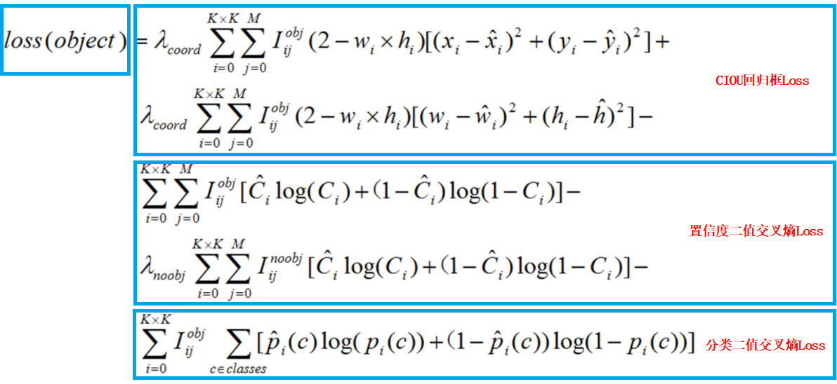
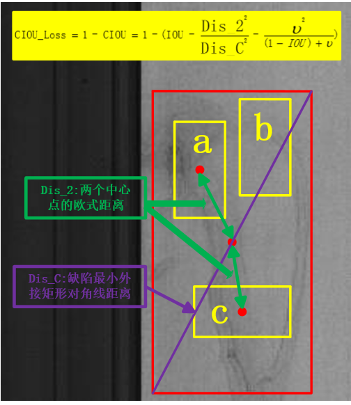
CIOU_Loss是创新点,与GIOU_Loss相比,引入了重叠面积与中心点的距离Dis_2来区分预测框a与b的定位差异,同时还引入了预测框和目标框的长宽比一致性因子ν,将a与c这种重叠面积与中心点距离相同但长宽比与目标框适配程度有差异的预测框区分开来,如图:

计算好Loss需要update_network():

复制代码
void update_network(network net)
{
    int i;
    int update_batch = net.batch*net.subdivisions;
    float rate = get_current_rate(net);
    for(i = 0; i < net.n; ++i){
        layer l = net.layers[i];
        if(l.update){
            l.update(l, update_batch, rate, net.momentum, net.decay); // convolutional_layer.c中,l.update = update_convolutional_layer。
        }
    }
}
复制代码

update_convolutional_layer()函数:

复制代码
void update_convolutional_layer(convolutional_layer l, int batch, float learning_rate_init, float momentum, float decay)
{
    float learning_rate = learning_rate_init*l.learning_rate_scale;
    axpy_cpu(l.nweights, -decay*batch, l.weights, 1, l.weight_updates, 1); // blas.c中,axpy_cpu函数入口,for(i = 0; i < l.nweights; ++i),l.weight_updates[i*1] -= decay*batch*l.weights[i*1]。
    axpy_cpu(l.nweights, learning_rate / batch, l.weight_updates, 1, l.weights, 1); // for(i = 0; i < l.nweights; ++i),l.weights[i*1] += (learning_rate/batch)*l.weight_updates[i*1]
    scal_cpu(l.nweights, momentum, l.weight_updates, 1); // blas.c中,scal_cpu函数入口,for(i = 0; i < l.nweights; ++i),l.weight_updates[i*1] *= momentum。
    axpy_cpu(l.n, learning_rate / batch, l.bias_updates, 1, l.biases, 1); // for(i = 0; i < l.n; ++i),l.biases[i*1] += (learning_rate/batch)*l.bias_updates[i*1]。
    scal_cpu(l.n, momentum, l.bias_updates, 1); // for(i = 0; i < l.n; ++i),l.bias_updates[i*1] *= momentum。
    if (l.scales) {
        axpy_cpu(l.n, learning_rate / batch, l.scale_updates, 1, l.scales, 1);
        scal_cpu(l.n, momentum, l.scale_updates, 1);
    }
}
复制代码

同样,在network_kernels.cu里,有GPU模式下的forward&backward相关的函数,涉及数据格式转换及加速,此处只讨论原理,暂时忽略GPU部分的代码。

复制代码
void forward_backward_network_gpu(network net, float *x, float *y)
{
......
    forward_network_gpu(net, state); // 正向。
    backward_network_gpu(net, state); // 反向。
......
}
复制代码

CPU模式下,采用带momentum的常规GD更新weights,同时在network.c中也提供了也提供了train_network_sgd()函数接口;GPU模式提供了adam选项,convolutional_layer.c中make_convolutional_layer()函数有体现。

七. 调参总结

本人在实际项目中涉及的是工业中的钢铁表面缺陷检测场景,不到2000张图片,3类,数据量很少。理论上YOLO系列并不太适合缺陷检测的问题,基于分割+分类的网络、Cascade-RCNN等或许是更好的选择,但我本着实验的态度,进行了多轮的训练和对比,整体上效果还是不错的。

1.max_batches: AlexeyAB在github工程上有提到,类别数*2000作为参考,不要少于6000,但这个是使用预训练权重的情况。如果train from scratch,要适当增加,具体要看你的数据情况,网络需要额外的时间来从零开始学习;

2.pretrain or not:当数据量很少时,预训练确实能更快使模型收敛,效果也不错,但缺陷检测这类问题,缺陷目标特征本身的特异性还是比较强的,虽然我的数据量也很少,但scratch的方式还是能取得稍好一些的效果;

3.anchors:cfg文件默认的anchors是基于COCO数据集,可以说尺度比较均衡,使用它效果不会差,但如果你自己的数据在尺度分布上不太均衡,建议自行生成新的anchors,可以直接使用源码里面的脚本,注意,要根据生成anchors的size(1-yolo:<30*30,2-yolo:<60*60,3-yolo:others)来改变索引值masks以及前一个conv层的filters参数;

4.rotate:YOLO-V4在目标检测这一块,其实没有用到旋转来进行数据增强,因此我在线下对数量最少的一个类进行了180旋转对称增强,该类样本数扩增一倍,效果目前还不明显,可能是数据量增加的还是太少,而且我还在训练对比,完成后可以补充;

5.mosaic:马赛克数据增强是必须要有的,mAP值提升比较明显,需要安装opencv,且和cutmix不能同时使用。

为什么从 MVC 到 DDD,架构的本质是什么? - 小傅哥 - 博客园

mikel阅读(821)

来源: 为什么从 MVC 到 DDD,架构的本质是什么? – 小傅哥 – 博客园

本文来自于小傅哥新编写的《Java简明教程》系列内容,本教程意在于通过简单、明了、清晰的成体系内容,教会Java学习伙伴,可以在学习后能进行Java项目开发。

今天要分享的是 MVC 和 DDD 的架构本质,通过由浅入深的介绍讲解和视频带着手把手操作创建工程架构。让无论是学习 MVC 的小白码农还是希望了解更多关于 DDD 内容的老白码农,都可以学习到一点自己需要的内容。

一、MVC 架构

如果我们尝试把编程的复杂架构缩小到最容易理解的程度,那么编程开发其实只做3件事:”定义属性创建方法调用展示“。但因为同类所需的内容较多,如一系列的属性,一堆的方法实现,一组的接口封装,那么就需要合理的把这些内容分配到不同的层次中去实现,因此有了分层架构的设计。

那么本文小傅哥会向大家介绍一套MVC架构的分层设计以及如何创建使用,并提供相应的简单的案例。你可以复制这套架构在自己的场景中使用,也更能方便编程的小白可以更快的上手开发。

注意:此套MVC架构模型适合提供HTTP服务的工程架构,适合简单的小场景开发使用。特点;轻便、简单、学习成本低。

1. 编程三步

如果说你是一个特别小的玩具项目,你甚至可以把编程的3步写到一个类里。但因为你做的是正经项目,你的各种类;对象类、库表类、方法类,就会成群结队的来。如果你想把这些成群结队的类的内容,都写到一个类里去,那么就是几万行的代码了。—— 当然你也可以吹牛逼,你一个人做过一个项目,这项目大到啥程度呢。就是有一个类里有上万行代码。

所以,为了不至于让一个类撑到爆💥,需要把黄色的对象、绿色的方法、红色的接口,都分配到不同的包结构下。这就是你编码人生中所接触到的第一个解耦操作。

2. 分层框架

MVC 是一种非常常见且常用的分层架构,主要包括;M – mode 对象层,封装到 domain 里。V – view 展示层,但因为目前都是前后端分离的项目,几乎不会在后端项目里写 JSP 文件了。C – Controller 控制层,对外提供接口实现类。DAO 算是单独拿出来用户处理数据库操作的层。

  • 如图,在 MVC 的分层架构下。我们编程3步的所需各类对象、方法、接口,都分配到 MVC 的各个层次中去。
  • 因为这样分层以后,就可以很清晰明了的知道各个层都在做什么内容,也更加方便后续的维护和迭代。
  • 对于一个真正的项目来说,是没有一锤子买卖的,最开始的开发远不是成本所在。最大的开发成本是后期的维护和迭代。而架构设计的意义更多的就是在解决系统的反复的维护和迭代时,如何降低成本,这也是架构分层的意义所在。

3. 调用流程

接下来我们再看下一套 MVC 架构中各个模块在调用时的串联关系;

  • 以用户发起 HTTP 请求开始,Controller 在接收到请求后,调用由 Spring 注入到类里的 Service 方法,进入 Service 方法后有些逻辑会走数据库,有些逻辑是直接内部自己处理后就直接返回给 Controller 了。最后由 Controller 封装结果返回给 HTTP 响应。
  • 同时我们也可以看到各个对象在这些请求间的一个作用,如;请求对象、库表对象、返回对象。

4. 架构源码

4.1 环境

  • JDK 1.8
  • Maven 3.8.6 – 下载安装maven后,本地记得配置阿里云镜像,方便快速拉取jar包。源码中 docs/maven/settings.xml 有阿里云镜像地址。
  • SpringBoot 2.7.2
  • MySQL 5.7 – 如果你使用 8.0 记得更改 pom.xml 中的 mySQL 引用

4.2 架构

.
├── docs
│   └── mvc.drawio - 架构文档
├── pom.xml
├── src
│   ├── main
│   │   ├── java
│   │   │   └── cn
│   │   │       └── bugstack
│   │   │           └── xfg
│   │   │               └── frame
│   │   │                   ├── Application.java
│   │   │                   ├── common
│   │   │                   │   ├── Constants.java
│   │   │                   │   └── Result.java
│   │   │                   ├── controller
│   │   │                   │   └── UserController.java
│   │   │                   ├── dao
│   │   │                   │   └── IUserDao.java
│   │   │                   ├── domain
│   │   │                   │   ├── po
│   │   │                   │   │   └── User.java
│   │   │                   │   ├── req
│   │   │                   │   │   └── UserReq.java
│   │   │                   │   ├── res
│   │   │                   │   │   └── UserRes.java
│   │   │                   │   └── vo
│   │   │                   │       └── UserInfo.java
│   │   │                   └── service
│   │   │                       ├── IUserService.java
│   │   │                       └── impl
│   │   │                           └── UserServiceImpl.java
│   │   └── resources
│   │       ├── application.yml
│   │       └── mybatis
│   │           ├── config
│   │           │   └── mybatis-config.xml
│   │           └── mapper
│   │               └── User_Mapper.xml
│   └── test
│       └── java
│           └── cn
│               └── bugstack
│                   └── xfg
│                       └── frame
│                           └── test
│                               └── ApiTest.java
└── road-map.sql

以上是整个🏭工程架构的 tree 树形图。整个工程由 SpringBoot 驱动。

  • Application.java 是启动程序的 SpringBoot 应用
  • common 是额外添加的一个层,用于定义通用的类
  • controller 控制层,提供接口实现。
  • dao 数据库操作层
  • domain 对象定义层
  • service 服务实现层

5. 测试验证

  • 首先;整个工程由 SpringBoot 驱动,提供了 road-map.sql 测试 SQL 库表语句。你可以在自己的本地mysql上进行执行。它会创建库表。
  • 之后;在 application.yml 配置数据库链接信息。
  • 之后就可以打开 ApiTest 进行测试了。你可以点击 Application 类的绿色箭头启动工程,使用 UserController 类提供接口的方式调用程序;http://localhost:8089/queryUserInfo

– 如果你正常获取了这样的结果信息,那么说明你已经启动成功。接下来就可以对照着MVC的结构进行学习,以及使用这样的工程结构开发自己的项目。

二、DDD 架构

从最早接触 DDD 架构,到后来用 DDD 架构不断的承接项目开发,一次次在项目开发中的经验积累。对 DDD 有了不少的理解。DDD 是一种思想,落地的形态和结构会有不同的方式,甚至在编码上也会有风格的差异。但终期目标就一个;”提供代码的可维护性,降低迭代开发成本。“也是康威定律所述:”任何组织在设计一套系统时,所交付的设计方案在结构上都与该组织的沟通结构保持一致。“

但 DDD 与 MVC 相比的概率较多,贸然用理论驱动代码开发,会让整个工程变得非常混乱,甚至可能虽然是用的 DDD 但最后写出来了一片四不像的 MVC 代码。所以对于程序员👨🏻‍💻来说,先能上手一个工程,在从工程了解理论会更加容易。为此小傅哥想以此文,通过实战编码的方式向大家分享 DDD 架构,并能让大家上手的 DDD 架构。

1. 问题碰撞

你用 MVC 写代码,遇到过最大的问题是什么?🤔

简单、容易、好理解,是 MVC 架构的特点,但也正因为简单的分层逻辑,在适配较复杂的场景并且需要长周期的维护时,代码的迭代成本就会越来越高。如图;

  • 如果你接触过较大型且已经长期维护项目的 MVC 架构,你就会发现这里的 DAO、PO、VO 对象,在 Service 层相互调用。那么长期开发后,就导致了各个 PO 里的属性字段数量都被撑的特别大。这样的开发方式,将”状态”“行为“分离到不同的对象中,代码的意图渐渐模糊,膨胀、臃肿和不稳定的架构,让迭代成本增加。
  • 而 DDD 架构首先以解决此类问题为主,将各个属于自己领域范围内的行为和逻辑封装到自己的领域包下处理。这也是 DDD 架构设计的精髓之一。它希望在分治层面合理切割问题空间为更小规模的若干子问题,而问题越小就容易被理解和处理,做到高内聚低耦合。这也是康威定律所提到的,解决复杂场景的设计主要分为:分治、抽象和知识。

2. 简化理解

在给大家讲解 MVC 架构的时候,小傅哥提到了一个简单的开发模型。开发代码可以理解为:“定义属性 -> 创建方法 -> 调用展示”但这个模型结构过于简单,不太适合运用了各类分布式技术栈以及更多逻辑的 DDD 架构。所以在 DDD 这里,我们把开发代码可以抽象为:“触发 -> 函数 -> 连接” 如图;

  • DDD 架构常用于微服务场景,因此也一个系统的调用方式就不只是 HTTP 还包括;RPC 远程MQ 消息TASK 任务,因此这些种方式都可以理解为触发。
  • 通过触发调用函数方法,我们这里可以把各个服务都当成一个函数方法来看。而函数方法通过连接,调用到其他的接口、数据库、缓存来完成函数逻辑。

接下来,小傅哥在带着大家把这些所需的模块,拆分到对应的DDD系统架构中。

3. 架构分层

如下是 DDD 架构的一种分层结构,也可以有其他种方式,核心的重点在于适合你所在场景的业务开发。以下的分层结构,是小傅哥在使用 DDD 架构多种的方式开发代码后,做了简化和处理的。右侧的连线是各个模块的依赖关系。接下来小傅哥就给大家做一下模块的介绍。

  • 接口定义 – xfg-frame-api:因为微服务中引用的 RPC 需要对外提供接口的描述信息,也就是调用方在使用的时候,需要引入 Jar 包,让调用方好能依赖接口的定义做代理。
  • 应用封装 – xfg-frame-app:这是应用启动和配置的一层,如一些 aop 切面或者 config 配置,以及打包镜像都是在这一层处理。你可以把它理解为专门为了启动服务而存在的。
  • 领域封装 – xfg-frame-domain:领域模型服务,是一个非常重要的模块。无论怎么做DDD的分层架构,domain 都是肯定存在的。在一层中会有一个个细分的领域服务,在每个服务包中会有【模型、仓库、服务】这样3部分。
  • 仓储服务 – xfg-frame-infrastructure:基础层依赖于 domain 领域层,因为在 domain 层定义了仓储接口需要在基础层实现。这是依赖倒置的一种设计方式。
  • 领域封装 – xfg-frame-trigger:触发器层,一般也被叫做 adapter 适配器层。用于提供接口实现、消息接收、任务执行等。所以对于这样的操作,小傅哥把它叫做触发器层。
  • 类型定义 – xfg-frame-types:通用类型定义层,在我们的系统开发中,会有很多类型的定义,包括;基本的 Response、Constants 和枚举。它会被其他的层进行引用使用。
  • 领域编排【可选】 – xfg-frame-case:领域编排层,一般对于较大且复杂的的项目,为了更好的防腐和提供通用的服务,一般会添加 case/application 层,用于对 domain 领域的逻辑进行封装组合处理。

4. 架构源码

4.1 环境

  • JDK 1.8
  • Maven 3.8.6
  • SpringBoot 2.7.2
  • MySQL 5.7 – 如果你使用 8.0 记得更改 pom.xml 中的 mysql 引用

4.2 架构

.
├── README.md
├── docs
│   ├── dev-ops
│   │   ├── environment
│   │   │   └── environment-docker-compose.yml
│   │   ├── siege.sh
│   │   └── skywalking
│   │       └── skywalking-docker-compose.yml
│   ├── doc.md
│   ├── sql
│   │   └── road-map.sql
│   └── xfg-frame-ddd.drawio
├── pom.xml
├── xfg-frame-api
│   ├── pom.xml
│   ├── src
│   │   └── main
│   │       └── java
│   │           └── cn
│   │               └── bugstack
│   │                   └── xfg
│   │                       └── frame
│   │                           └── api
│   │                               ├── IAccountService.java
│   │                               ├── IRuleService.java
│   │                               ├── model
│   │                               │   ├── request
│   │                               │   │   └── DecisionMatterRequest.java
│   │                               │   └── response
│   │                               │       └── DecisionMatterResponse.java
│   │                               └── package-info.java
│   └── xfg-frame-api.iml
├── xfg-frame-app
│   ├── Dockerfile
│   ├── build.sh
│   ├── pom.xml
│   ├── src
│   │   ├── main
│   │   │   ├── bin
│   │   │   │   ├── start.sh
│   │   │   │   └── stop.sh
│   │   │   ├── java
│   │   │   │   └── cn
│   │   │   │       └── bugstack
│   │   │   │           └── xfg
│   │   │   │               └── frame
│   │   │   │                   ├── Application.java
│   │   │   │                   ├── aop
│   │   │   │                   │   ├── RateLimiterAop.java
│   │   │   │                   │   └── package-info.java
│   │   │   │                   └── config
│   │   │   │                       ├── RateLimiterAopConfig.java
│   │   │   │                       ├── RateLimiterAopConfigProperties.java
│   │   │   │                       ├── ThreadPoolConfig.java
│   │   │   │                       ├── ThreadPoolConfigProperties.java
│   │   │   │                       └── package-info.java
│   │   │   └── resources
│   │   │       ├── application-dev.yml
│   │   │       ├── application-prod.yml
│   │   │       ├── application-test.yml
│   │   │       ├── application.yml
│   │   │       ├── logback-spring.xml
│   │   │       └── mybatis
│   │   │           ├── config
│   │   │           │   └── mybatis-config.xml
│   │   │           └── mapper
│   │   │               ├── RuleTreeNodeLine_Mapper.xml
│   │   │               ├── RuleTreeNode_Mapper.xml
│   │   │               └── RuleTree_Mapper.xml
│   │   └── test
│   │       └── java
│   │           └── cn
│   │               └── bugstack
│   │                   └── xfg
│   │                       └── frame
│   │                           └── test
│   │                               └── ApiTest.java
│   └── xfg-frame-app.iml
├── xfg-frame-ddd.iml
├── xfg-frame-domain
│   ├── pom.xml
│   ├── src
│   │   └── main
│   │       └── java
│   │           └── cn
│   │               └── bugstack
│   │                   └── xfg
│   │                       └── frame
│   │                           └── domain
│   │                               ├── order
│   │                               │   ├── model
│   │                               │   │   ├── aggregates
│   │                               │   │   │   └── OrderAggregate.java
│   │                               │   │   ├── entity
│   │                               │   │   │   ├── OrderItemEntity.java
│   │                               │   │   │   └── ProductEntity.java
│   │                               │   │   ├── package-info.java
│   │                               │   │   └── valobj
│   │                               │   │       ├── OrderIdVO.java
│   │                               │   │       ├── ProductDescriptionVO.java
│   │                               │   │       └── ProductNameVO.java
│   │                               │   ├── repository
│   │                               │   │   ├── IOrderRepository.java
│   │                               │   │   └── package-info.java
│   │                               │   └── service
│   │                               │       ├── OrderService.java
│   │                               │       └── package-info.java
│   │                               ├── rule
│   │                               │   ├── model
│   │                               │   │   ├── aggregates
│   │                               │   │   │   └── TreeRuleAggregate.java
│   │                               │   │   ├── entity
│   │                               │   │   │   ├── DecisionMatterEntity.java
│   │                               │   │   │   └── EngineResultEntity.java
│   │                               │   │   ├── package-info.java
│   │                               │   │   └── valobj
│   │                               │   │       ├── TreeNodeLineVO.java
│   │                               │   │       ├── TreeNodeVO.java
│   │                               │   │       └── TreeRootVO.java
│   │                               │   ├── repository
│   │                               │   │   ├── IRuleRepository.java
│   │                               │   │   └── package-info.java
│   │                               │   └── service
│   │                               │       ├── engine
│   │                               │       │   ├── EngineBase.java
│   │                               │       │   ├── EngineConfig.java
│   │                               │       │   ├── EngineFilter.java
│   │                               │       │   └── impl
│   │                               │       │       └── RuleEngineHandle.java
│   │                               │       ├── logic
│   │                               │       │   ├── BaseLogic.java
│   │                               │       │   ├── LogicFilter.java
│   │                               │       │   └── impl
│   │                               │       │       ├── UserAgeFilter.java
│   │                               │       │       └── UserGenderFilter.java
│   │                               │       └── package-info.java
│   │                               └── user
│   │                                   ├── model
│   │                                   │   └── valobj
│   │                                   │       └── UserVO.java
│   │                                   ├── repository
│   │                                   │   └── IUserRepository.java
│   │                                   └── service
│   │                                       ├── UserService.java
│   │                                       └── impl
│   │                                           └── UserServiceImpl.java
│   └── xfg-frame-domain.iml
├── xfg-frame-infrastructure
│   ├── pom.xml
│   ├── src
│   │   └── main
│   │       └── java
│   │           └── cn
│   │               └── bugstack
│   │                   └── xfg
│   │                       └── frame
│   │                           └── infrastructure
│   │                               ├── dao
│   │                               │   ├── IUserDao.java
│   │                               │   ├── RuleTreeDao.java
│   │                               │   ├── RuleTreeNodeDao.java
│   │                               │   └── RuleTreeNodeLineDao.java
│   │                               ├── package-info.java
│   │                               ├── po
│   │                               │   ├── RuleTreeNodeLineVO.java
│   │                               │   ├── RuleTreeNodeVO.java
│   │                               │   ├── RuleTreeVO.java
│   │                               │   └── UserPO.java
│   │                               └── repository
│   │                                   ├── RuleRepository.java
│   │                                   └── UserRepository.java
│   └── xfg-frame-infrastructure.iml
├── xfg-frame-trigger
│   ├── pom.xml
│   ├── src
│   │   └── main
│   │       └── java
│   │           └── cn
│   │               └── bugstack
│   │                   └── xfg
│   │                       └── frame
│   │                           └── trigger
│   │                               ├── http
│   │                               │   ├── Controller.java
│   │                               │   └── package-info.java
│   │                               ├── mq
│   │                               │   └── package-info.java
│   │                               ├── rpc
│   │                               │   ├── AccountService.java
│   │                               │   ├── RuleService.java
│   │                               │   └── package-info.java
│   │                               └── task
│   │                                   └── package-info.java
│   └── xfg-frame-trigger.iml
└── xfg-frame-types
    ├── pom.xml
    ├── src
    │   └── main
    │       └── java
    │           └── cn
    │               └── bugstack
    │                   └── xfg
    │                       └── frame
    │                           └── types
    │                               ├── Constants.java
    │                               ├── Response.java
    │                               └── package-info.java
    └── xfg-frame-types.iml

以上是整个🏭工程架构的 tree 树形图。整个工程由 xfg-frame-app 模的 SpringBoot 驱动。这里小傅哥在 domain 领域模型下提供了 order、rule、user 三个领域模块。并在每个模块下提供了对应的测试内容。这块是整个模型的重点,其他模块都可以通过测试看到这里的调用过程。

4.3 领域

一个领域模型中包含3个部分;model、repository、service 三部分;

  • model 对象的定义
  • repository 仓储的定义
  • service 服务实现

以上3个模块,一般也是大家在使用 DDD 时候最不容易理解的分层。比如 model 里还分为;valobj – 值对象、entity 实体对象、aggregates 聚合对象;

  • 值对象:表示没有唯一标识的业务实体,例如商品的名称、描述、价格等。
  • 实体对象:表示具有唯一标识的业务实体,例如订单、商品、用户等;
  • 聚合对象:是一组相关的实体对象的根,用于保证实体对象之间的一致性和完整性;

关于model中各个对象的拆分,尤其是聚合的定义,会牵引着整个模型的设计。当然你可以在初期使用 DDD 的时候不用过分在意领域模型的设计,可以把整个 domain 下的一个个包当做充血模型结构,这样编写出来的代码也是非常适合维护的。

4.4 环境(开发/测试/上线)

源码xfg-frame-ddd/pom.xml

<profile>
    <id>dev</id>
    <activation>
        <activeByDefault>true</activeByDefault>
    </activation>
    <properties>
        <profileActive>dev</profileActive>
    </properties>
</profile>
<profile>
    <id>test</id>
    <properties>
        <profileActive>test</profileActive>
    </properties>
</profile>
<profile>
    <id>prod</id>
    <properties>
        <profileActive>prod</profileActive>
    </properties>
</profile>
  • 定义环境;开发、测试、上线。

源码xfg-frame-app/application.yml

spring:
  config:
    name: xfg-frame
  profiles:
    active: dev # dev、test、prod
  • 除了 pom 的配置,还需要在 application.yml 中指定环境。这样就可以对应的加载到;application-dev.ymlapplication-prod.ymlapplication-test.yml 这样就可以很方便的加载对应的配置信息了。尤其是各个场景中切换会更加方便。

4.5 切面

一个工程开发中,有时候可能会有很多的统一切面和启动配置的处理,这些内容都可以在 xfg-frame-app 完成。

源码cn.bugstack.xfg.frame.aop.RateLimiterAop

@Slf4j
@Aspect
public class RateLimiterAop {

    private final long timeout;
    private final double permitsPerSecond;
    private final RateLimiter limiter;

    public RateLimiterAop(double permitsPerSecond, long timeout) {
        this.permitsPerSecond = permitsPerSecond;
        this.timeout = timeout;
        this.limiter = RateLimiter.create(permitsPerSecond);
    }

    @Pointcut("execution(* cn.bugstack.xfg.frame.trigger..*.*(..))")
    public void pointCut() {
    }

    @Around(value = "pointCut()", argNames = "jp")
    public Object around(ProceedingJoinPoint jp) throws Throwable {
        boolean tryAcquire = limiter.tryAcquire(timeout, TimeUnit.MILLISECONDS);
        if (!tryAcquire) {
            Method method = getMethod(jp);
            log.warn("方法 {}.{} 请求已被限流,超过限流配置[{}/秒]", method.getDeclaringClass().getCanonicalName(), method.getName(), permitsPerSecond);
            return Response.<Object>builder()
                    .code(Constants.ResponseCode.RATE_LIMITER.getCode())
                    .info(Constants.ResponseCode.RATE_LIMITER.getInfo())
                    .build();
        }
        return jp.proceed();
    }

    private Method getMethod(JoinPoint jp) throws NoSuchMethodException {
        Signature sig = jp.getSignature();
        MethodSignature methodSignature = (MethodSignature) sig;
        return jp.getTarget().getClass().getMethod(methodSignature.getName(), methodSignature.getParameterTypes());
    }

}

使用

# 限流配置
rate-limiter:
  permits-per-second: 1
  timeout: 5
  • 这样你所有的通用配置,又和业务没有太大的关系的,就可以直接写到这里了。—— 具体可以参考代码。

5. 测试验证

  • 首先;整个工程由 SpringBoot 驱动,提供了 road-map.sql 测试 SQL 库表语句。你可以在自己的本地mysql上进行执行。它会创建库表。
  • 之后;在 application.yml 配置数据库链接信息。
  • 之后就可以打开 ApiTest 进行测试了。你可以点击 Application 类的绿色箭头启动工程,使用触发器里的接口调用测试,或者单元测试RPC接口,小傅哥也提供了泛化调用的方式。
  • 如果你正常获取了这样的结果信息,那么说明你已经启动成功。接下来就可以对照着DDD的结构进行学习,以及使用这样的工程结构开发自己的项目。

三、实战 – DDD 项目

纸上得来终觉浅,码农学习要实战!

无论是 MVC 还是各类 DDD 所呈现的架构,还是需要看到实际的代码,以及参与实战开发才能更好的吸收。否则都是理论仍旧难以让人下手。

所以小傅哥为大家准备了一些学习项目,这些项目都是非常具有架构思维以及设计模式的应用级实战项目架构设计和落地。对于一些小白来说,如果能早早的接触到这样的项目,就相当于是提前进入企业实习了。可以极大的提到编程思维以及开发能力。

这些项目包括:《Lottery 抽奖系统 – 基于领域驱动设计的四层架构实践》、《API网关:中间件设计和落地》、《ChatGPT 微服务应用体系搭建》、《IM 仿微信》、《SpringBoot Starter 中间件设计和落地》等。这里小傅哥只列3张图,你就知道有多牛皮了!

第1张:Lottery

架构

工程

第2张:API网关

架构

工程

第3张:ChatGPT


实战项目:https://bugstack.cn/md/zsxq/introduce.html

此外,小傅哥还给大家准备了一系列的《Java简明教程》视频,进入B站即可学习!

https://www.bilibili.com/video/BV1kV411g7GX

Vue3从入门到精通(三) - 明志德道 - 博客园

mikel阅读(816)

来源: Vue3从入门到精通(三) – 明志德道 – 博客园

vue3插槽Slots

在 Vue3 中,插槽(Slots)的使用方式与 Vue2 中基本相同,但有一些细微的差异。以下是在 Vue3 中使用插槽的示例:

// ChildComponent.vue
<template>
  <div>
    <h2>Child Component</h2>
    <slot></slot>
  </div>
</template>
​
// ParentComponent.vue
<template>
  <div>
    <h1>Parent Component</h1>
    <ChildComponent>
      <p>This is the content of the slot.</p>
    </ChildComponent>
  </div>
</template><script>
  import { defineComponent } from 'vue'
  import ChildComponent from './ChildComponent.vue'export default defineComponent({
    name: 'ParentComponent',
    components: {
      ChildComponent
    }
  })
</script>

在上面的示例中,ChildComponent 组件定义了一个默认插槽,使用 <slot></slot> 标签来表示插槽的位置。在 ParentComponent 组件中,使用 <ChildComponent> 标签包裹了一段内容 <p>This is the content of the slot.</p>,这段内容将被插入到 ChildComponent 组件的插槽位置。

需要注意的是,在 Vue3 中,默认插槽不再具有具名插槽的概念。如果需要使用具名插槽,可以使用 v-slot 指令。以下是一个示例:

// ChildComponent.vue
<template>
  <div>
    <h2>Child Component</h2>
    <slot name="header"></slot>
    <slot></slot>
    <slot name="footer"></slot>
  </div>
</template>
​
// ParentComponent.vue
<template>
  <div>
    <h1>Parent Component</h1>
    <ChildComponent>
      <template v-slot:header>
        <h3>This is the header slot</h3>
      </template>
      <p>This is the content of the default slot.</p>
      <template v-slot:footer>
        <p>This is the footer slot</p>
      </template>
    </ChildComponent>
  </div>
</template><script>
  import { defineComponent } from 'vue'
  import ChildComponent from './ChildComponent.vue'export default defineComponent({
    name: 'ParentComponent',
    components: {
      ChildComponent
    }
  })
</script>

在上面的示例中,ChildComponent 组件定义了三个插槽,分别是名为 header、默认插槽和名为 footer 的插槽。在 ParentComponent 组件中,使用 <template v-slot:header> 来定义 header 插槽的内容,使用 <template v-slot:footer> 来定义 footer 插槽的内容。默认插槽可以直接写在组件标签内部。

需要注意的是,在 Vue3 中,v-slot 只能用在 <template> 标签上,不能用在普通的 HTML 标签上。如果要在普通 HTML 标签上使用插槽,可以使用 v-slot 的缩写语法 #。例如,<template v-slot:header> 可以简写为 #header

vue3组件生命周期

在 Vue3 中,组件的生命周期钩子函数与 Vue2 中有一些变化。以下是 Vue3 中常用的组件生命周期钩子函数:

  1. beforeCreate: 在实例初始化之后、数据观测之前被调用。

  2. created: 在实例创建完成之后被调用。此时,实例已完成数据观测、属性和方法的运算,但尚未挂载到 DOM 中。

  3. beforeMount: 在挂载开始之前被调用。在此阶段,模板已经编译完成,但尚未将模板渲染到 DOM 中。

  4. mounted: 在挂载完成之后被调用。此时,组件已经被挂载到 DOM 中,可以访问到 DOM 元素。

  5. beforeUpdate: 在数据更新之前被调用。在此阶段,虚拟 DOM 已经重新渲染,并将计算得到的变化应用到真实 DOM 上,但尚未更新到视图中。

  6. updated: 在数据更新之后被调用。此时,组件已经更新到最新的状态,DOM 也已经更新完成。

  7. beforeUnmount: 在组件卸载之前被调用。在此阶段,组件实例仍然可用,可以访问到组件的数据和方法。

  8. unmounted: 在组件卸载之后被调用。此时,组件实例已经被销毁,无法再访问到组件的数据和方法。

需要注意的是,Vue3 中移除了一些生命周期钩子函数,如 beforeDestroy 和 destroyed。取而代之的是 beforeUnmount 和 unmounted

另外,Vue3 中还引入了新的生命周期钩子函数 onRenderTracked 和 onRenderTriggered,用于追踪组件的渲染过程和触发的依赖项。

需要注意的是,Vue3 推荐使用 Composition API 来编写组件逻辑,而不是依赖于生命周期钩子函数。Composition API 提供了 setup 函数,用于组件的初始化和逻辑组织。在 setup 函数中,可以使用 onBeforeMountonMountedonBeforeUpdateonUpdatedonBeforeUnmount 等函数来替代相应的生命周期钩子函数。

vue3生命周期应用

Vue3 的生命周期钩子函数可以用于在组件的不同生命周期阶段执行相应的操作。以下是一些 Vue3 生命周期的应用场景示例:

  1. beforeCreate 和 created:在组件实例创建之前和创建之后执行一些初始化操作,如设置初始数据、进行异步请求等。

export default {
  beforeCreate() {
    console.log('beforeCreate hook');
    // 执行一些初始化操作
  },
  created() {
    console.log('created hook');
    // 执行一些初始化操作
  },
};
  1. beforeMount 和 mounted:在组件挂载之前和挂载之后执行一些 DOM 操作,如获取 DOM 元素、绑定事件等。

export default {
  beforeMount() {
    console.log('beforeMount hook');
    // 执行一些 DOM 操作
  },
  mounted() {
    console.log('mounted hook');
    // 执行一些 DOM 操作
  },
};
  1. beforeUpdate 和 updated:在组件数据更新之前和更新之后执行一些操作,如更新 DOM、发送请求等。

export default {
  beforeUpdate() {
    console.log('beforeUpdate hook');
    // 执行一些操作
  },
  updated() {
    console.log('updated hook');
    // 执行一些操作
  },
};
  1. beforeUnmount 和 unmounted:在组件卸载之前和卸载之后执行一些清理操作,如取消订阅、清除定时器等。

export default {
  beforeUnmount() {
    console.log('beforeUnmount hook');
    // 执行一些清理操作
  },
  unmounted() {
    console.log('unmounted hook');
    // 执行一些清理操作
  },
};

这些示例展示了 Vue3 生命周期钩子函数的一些常见应用场景。根据具体需求,你可以在相应的生命周期钩子函数中执行适当的操作。

vue3动态组件

在 Vue3 中,可以使用动态组件来根据不同的条件或状态动态地渲染不同的组件。使用动态组件可以使应用更加灵活和可扩展。以下是使用动态组件的示例:

  1. 使用 component 元素和 :is 属性来实现动态组件的渲染:

<template>
  <div>
    <component :is="currentComponent"></component>
    <button @click="toggleComponent">Toggle Component</button>
  </div>
</template><script>
import ComponentA from './ComponentA.vue';
import ComponentB from './ComponentB.vue';export default {
  data() {
    return {
      currentComponent: 'ComponentA',
    };
  },
  methods: {
    toggleComponent() {
      this.currentComponent = this.currentComponent === 'ComponentA' ? 'ComponentB' : 'ComponentA';
    },
  },
  components: {
    ComponentA,
    ComponentB,
  },
};
</script>

在上面的示例中,根据 currentComponent 的值动态地渲染 ComponentA 或 ComponentB 组件。点击按钮时,切换 currentComponent 的值,从而实现动态组件的切换。

  1. 使用 v-if 和 v-else 来根据条件渲染不同的组件:

<template>
  <div>
    <component-a v-if="showComponentA"></component-a>
    <component-b v-else></component-b>
    <button @click="toggleComponent">Toggle Component</button>
  </div>
</template><script>
import ComponentA from './ComponentA.vue';
import ComponentB from './ComponentB.vue';export default {
  data() {
    return {
      showComponentA: true,
    };
  },
  methods: {
    toggleComponent() {
      this.showComponentA = !this.showComponentA;
    },
  },
  components: {
    ComponentA,
    ComponentB,
  },
};
</script>

在上面的示例中,根据 showComponentA 的值使用 v-if 和 v-else 来渲染 ComponentA 或 ComponentB 组件。点击按钮时,切换 showComponentA 的值,从而实现动态组件的切换。

这些示例演示了在 Vue3 中如何使用动态组件来根据条件或状态动态地渲染不同的组件。你可以根据具体需求选择适合的方式来使用动态组件。

vue3组件保持存活

在 Vue3 中,可以使用 <keep-alive> 组件来保持组件的存活状态,即使组件在组件树中被切换或销毁,它的状态仍然会被保留。这对于需要在组件之间共享状态或缓存数据的场景非常有用。以下是使用 <keep-alive> 组件来保持组件存活的示例:

<template>
  <div>
    <button @click="toggleComponent">Toggle Component</button>
    <keep-alive>
      <component :is="currentComponent"></component>
    </keep-alive>
  </div>
</template><script>
import ComponentA from './ComponentA.vue';
import ComponentB from './ComponentB.vue';export default {
  data() {
    return {
      currentComponent: 'ComponentA',
    };
  },
  methods: {
    toggleComponent() {
      this.currentComponent = this.currentComponent === 'ComponentA' ? 'ComponentB' : 'ComponentA';
    },
  },
  components: {
    ComponentA,
    ComponentB,
  },
};
</script>

在上面的示例中,使用 <keep-alive> 组件将 <component> 包裹起来,这样在切换组件时,被包裹的组件的状态将会被保留。点击按钮时,切换 currentComponent 的值,从而切换要渲染的组件。

需要注意的是,被 <keep-alive> 包裹的组件在切换时会触发一些特定的生命周期钩子函数,如 activated 和 deactivated。你可以在这些钩子函数中执行一些特定的操作,如获取焦点、发送请求等。

<template>
  <div>
    <h2>Component A</h2>
  </div>
</template><script>
export default {
  activated() {
    console.log('Component A activated');
    // 执行一些操作
  },
  deactivated() {
    console.log('Component A deactivated');
    // 执行一些操作
  },
};
</script>

在上面的示例中,当组件 A 被激活或停用时,分别在 activated 和 deactivated 钩子函数中输出相应的信息。

使用 <keep-alive> 组件可以方便地保持组件的存活状态,并在组件之间共享状态或缓存数据。

vue3异步组件

在 Vue3 中,可以使用异步组件来延迟加载组件的代码,从而提高应用的性能和加载速度。异步组件在需要时才会被加载,而不是在应用初始化时就加载所有组件的代码。以下是使用异步组件的示例:

  1. 使用 defineAsyncComponent 函数来定义异步组件:

<template>
  <div>
    <button @click="loadComponent">Load Component</button>
    <component v-if="isComponentLoaded" :is="component"></component>
  </div>
</template><script>
import { defineAsyncComponent } from 'vue';const AsyncComponent = defineAsyncComponent(() =>
  import('./Component.vue')
);export default {
  data() {
    return {
      isComponentLoaded: false,
      component: null,
    };
  },
  methods: {
    loadComponent() {
      this.isComponentLoaded = true;
      this.component = AsyncComponent;
    },
  },
};
</script>

在上面的示例中,使用 defineAsyncComponent 函数来定义异步组件 AsyncComponent。当点击按钮时,设置 isComponentLoaded 为 true,并将 component 设置为 AsyncComponent,从而加载异步组件。

  1. 使用 Suspense 组件来处理异步组件的加载状态:

<template>
  <div>
    <Suspense>
      <template #default>
        <component :is="component"></component>
      </template>
      <template #fallback>
        <div>Loading...</div>
      </template>
    </Suspense>
    <button @click="loadComponent">Load Component</button>
  </div>
</template><script>
import { defineAsyncComponent, Suspense } from 'vue';const AsyncComponent = defineAsyncComponent(() =>
  import('./Component.vue')
);export default {
  data() {
    return {
      component: null,
    };
  },
  methods: {
    loadComponent() {
      this.component = AsyncComponent;
    },
  },
};
</script>

在上面的示例中,使用 Suspense 组件来处理异步组件的加载状态。在 default 插槽中,渲染异步组件,而在 fallback 插槽中,渲染加载状态的提示信息。当点击按钮时,加载异步组件。

这些示例演示了在 Vue3 中如何使用异步组件来延迟加载组件的代码。使用异步组件可以提高应用的性能和加载速度,特别是在应用中有大量组件时。

vue3依赖注入

在 Vue3 中,可以使用依赖注入来在组件之间共享数据或功能。Vue3 提供了 provide 和 inject 两个函数来实现依赖注入。

  1. 使用 provide 函数在父组件中提供数据或功能:

<template>
  <div>
    <ChildComponent></ChildComponent>
  </div>
</template><script>
import { provide } from 'vue';
import MyService from './MyService';export default {
  setup() {
    provide('myService', new MyService());
  },
};
</script>

在上面的示例中,使用 provide 函数在父组件中提供了一个名为 myService 的数据或功能,它的值是一个 MyService 的实例。

  1. 使用 inject 函数在子组件中注入提供的数据或功能:

<template>
  <div>
    <p>{{ message }}</p>
  </div>
</template><script>
import { inject } from 'vue';export default {
  setup() {
    const myService = inject('myService');
    const message = myService.getMessage();return {
      message,
    };
  },
};
</script>

在上面的示例中,使用 inject 函数在子组件中注入了父组件提供的名为 myService 的数据或功能。通过注入的 myService 实例,可以调用其中的方法或访问其中的属性。

通过使用 provide 和 inject 函数,可以在组件之间实现依赖注入,从而实现数据或功能的共享。这在多个组件需要访问相同的数据或功能时非常有用。

vue3应用

Vue3 是一个用于构建用户界面的现代化 JavaScript 框架。它具有响应式数据绑定、组件化、虚拟 DOM 等特性,使得开发者可以更高效地构建交互式的 Web 应用。

下面是一些使用 Vue3 开发应用的步骤:

  1. 安装 Vue3:使用 npm 或 yarn 安装 Vue3 的最新版本。

npm install vue@next
  1. 创建 Vue3 应用:创建一个新的 Vue3 项目。

vue create my-app
  1. 编写组件:在 src 目录下创建组件文件,例如 HelloWorld.vue

<template>
  <div>
    <h1>{{ message }}</h1>
    <button @click="changeMessage">Change Message</button>
  </div>
</template>
​
<script>
import { ref } from 'vue';
​
export default {
  setup() {
    const message = ref('Hello, Vue3!');
​
    const changeMessage = () => {
      message.value = 'Hello, World!';
    };
​
    return {
      message,
      changeMessage,
    };
  },
};
</script>

在上面的示例中,使用 ref 函数创建了一个响应式的数据 message,并在模板中使用它。通过点击按钮,可以改变 message 的值。

  1. 使用组件:在 App.vue 中使用自定义的组件。

<template>
  <div>
    <HelloWorld></HelloWorld>
  </div>
</template>
​
<script>
import HelloWorld from './components/HelloWorld.vue';
​
export default {
  components: {
    HelloWorld,
  },
};
</script>

在上面的示例中,导入并注册了自定义的 HelloWorld 组件,并在模板中使用它。

  1. 运行应用:在命令行中运行以下命令启动应用。

npm run serve

这将启动开发服务器,并在浏览器中打开应用。

这只是一个简单的示例,你可以根据实际需求编写更复杂的组件和应用逻辑。Vue3 还提供了许多其他功能和工具,如路由、状态管理、单文件组件等,以帮助你构建更强大的应用。

希望这个简单的示例能帮助你入门 Vue3 应用的开发!

献给转java的c#和java程序员的数据库orm框架 - 薛家明 - 博客园

mikel阅读(538)

来源: 献给转java的c#和java程序员的数据库orm框架 – 薛家明 – 博客园

献给转java的C#和java程序员的数据库orm框架

一个好的程序员不应被语言所束缚,正如我现在开源java的orm框架一样,如果您是一位转java的C#程序员,那么这个框架可以带给你起码没有那么差的业务编写和强类型体验。如果您是一位java程序员,那么该框架可以提供比Mybatis-Plus功能更加丰富、性能更高,更加轻量和完全免费的体验来做一个happy coding crud body。

背景

easy-query该框架是我在使用Mybatis-Plus(下面统称MP) 2年后开发的,因为MP不支持多表(不要提join插件(逻辑删除子表不支持)),并且Mybatis原本的xml十分恶心,导致项目中有非常多的代码需要编写SQL,并且整体数据库架构因为存在逻辑删除字段和多租户字段所以编写的SQL基本上多多少少都会有问题,我不相信大家没遇到过,而且MP得一些功能还需要收费这大大让我坚定还是自己开发一款。

介绍

easy-query 🚀 是一款无任何依赖的JAVA ORM 框架,十分轻量,拥有非常高的性能,支持单表查询、多表查询、union、子查询、分页、动态表名、VO对象查询返回、逻辑删、全局拦截、数据库列加密(支持高性能like查询)、数据追踪差异更新、乐观锁、多租户、自动分库、自动分表、读写分离,支持框架全功能外部扩展定制,拥有强类型表达式。

📚 文档

GITHUB地址 | GITEE地址

缺点

先说一下缺点,目前只适配了MySQL,不过基本上如果你是pgsql很少需要改动就直接可以用了,其他数据库可能因为自己的语法和特性会需要稍微做一下修改但是整体而言无需过多的变动,框架已经全部抽象好了。

功能点

  • 实体对象insert,update,delete全部支持
  • 单表查询、多表join查询,in子查询,exists子查询,连表统计(select a,(select count(1) from b) from c),联合查询union | all,分组group | having
  • 分页
  • 动态表名:运行时修改表名
  • 原生sql执行,查询
  • select查询map结果返回
  • select支持直接返回DTO对象实现自定义列查询返回,而不是全部列返回
  • select支持标记large字段不返回(默认返回)
  • 逻辑删除,自定义逻辑删除,支持多字段逻辑删除填充,支持运行时禁用
  • 全局拦截器,支持运行时选择性使用某几个或者不使用,支持entity操作 insert,update,条件拦截 select、update、delete的where条件拦截,update set字段拦截器
  • 多租户,支持表的列范围多租户模式
  • 数据库列加密,支持高性能的like模糊搜索匹配(不是单纯的调用数据库加密函数或者单纯的调用框架加密解密函数)
  • 数据追踪差异更新,而不是全列更新,用过efcore的肯定很熟悉
  • 版本号、乐观锁,支持自定义乐观锁
  • 支持分库分表(身为sharding-core作者不支持说不过去),全自动分库分表,仅需用户新增表和告知easy-query系统中有的表
  • 高性能分库分表分页,支持顺序分页,反向分页,支持高性能顺序分页和反向分页
  • 分库分表多字段分片
  • 分库分表自定义分片路由规则
  • 支持读写分离,一主多从支持分片下读写分离

目前项目正处于起步阶段后续会随着用户不断地完善各数据库的适配和功能的支持

开始使用

安装

以下是spring-boot环境和控制台模式的安装

spring-boot

<properties>
    <easy-query.version>0.8.10</easy-query.version>
</properties>
<dependency>
    <groupId>com.easy-query</groupId>
    <artifactId>sql-springboot-starter</artifactId>
    <version>${easy-query.version}</version>
</dependency>

console

以mysql为例

<properties>
    <easy-query.version>0.8.10</easy-query.version>
</properties>
<dependency>
    <groupId>com.easy-query</groupId>
    <artifactId>sql-mysql</artifactId>
    <version>${easy-query.version}</version>
</dependency>
//初始化连接池
 HikariDataSource dataSource = new HikariDataSource();
dataSource.setJdbcUrl("jdbc:mysql://127.0.0.1:3306/easy-query-test?serverTimezone=GMT%2B8&characterEncoding=utf-8&useSSL=false&allowMultiQueries=true&rewriteBatchedStatements=true");
dataSource.setUsername("root");
dataSource.setPassword("root");
dataSource.setDriverClassName("com.mysql.cj.jdbc.Driver");
dataSource.setMaximumPoolSize(20);
//创建easy-query
 EasyQuery easyQuery = EasyQueryBootstrapper.defaultBuilderConfiguration()
                .setDefaultDataSource(dataSource)
                .useDatabaseConfigure(new MySQLDatabaseConfiguration())
                .build();

开始

sql脚本

create table t_topic
(
    id varchar(32) not null comment '主键ID'primary key,
    stars int not null comment '点赞数',
    title varchar(50) null comment '标题',
    create_time datetime not null comment '创建时间'
)comment '主题表';

create table t_blog
(
    id varchar(32) not null comment '主键ID'primary key,
    deleted tinyint(1) default 0 not null comment '是否删除',
    create_by varchar(32) not null comment '创建人',
    create_time datetime not null comment '创建时间',
    update_by varchar(32) not null comment '更新人',
    update_time datetime not null comment '更新时间',
    title varchar(50) not null comment '标题',
    content varchar(256) null comment '内容',
    url varchar(128) null comment '博客链接',
    star int not null comment '点赞数',
    publish_time datetime null comment '发布时间',
    score decimal(18, 2) not null comment '评分',
    status int not null comment '状态',
    `order` decimal(18, 2) not null comment '排序',
    is_top tinyint(1) not null comment '是否置顶',
    top tinyint(1) not null comment '是否置顶'
)comment '博客表';

查询对象


@Data
public class BaseEntity implements Serializable {
    private static final long serialVersionUID = -4834048418175625051L;

    @Column(primaryKey = true)
    private String id;
    /**
     * 创建时间;创建时间
     */
    private LocalDateTime createTime;
    /**
     * 修改时间;修改时间
     */
    private LocalDateTime updateTime;
    /**
     * 创建人;创建人
     */
    private String createBy;
    /**
     * 修改人;修改人
     */
    private String updateBy;
    /**
     * 是否删除;是否删除
     */
    @LogicDelete(strategy = LogicDeleteStrategyEnum.BOOLEAN)
    private Boolean deleted;
}


@Data
@Table("t_topic")
@ToString
public class Topic {

    @Column(primaryKey = true)
    private String id;
    private Integer stars;
    private String title;
    private LocalDateTime createTime;
}

@Data
@Table("t_blog")
public class BlogEntity extends BaseEntity{

    /**
     * 标题
     */
    private String title;
    /**
     * 内容
     */
    private String content;
    /**
     * 博客链接
     */
    private String url;
    /**
     * 点赞数
     */
    private Integer star;
    /**
     * 发布时间
     */
    private LocalDateTime publishTime;
    /**
     * 评分
     */
    private BigDecimal score;
    /**
     * 状态
     */
    private Integer status;
    /**
     * 排序
     */
    private BigDecimal order;
    /**
     * 是否置顶
     */
    private Boolean isTop;
    /**
     * 是否置顶
     */
    private Boolean top;
}

单表查询

Topic topic = easyQuery
                .queryable(Topic.class)
                .where(o -> o.eq(Topic::getId, "3"))
                .firstOrNull();      
==> Preparing: SELECT t.`id`,t.`stars`,t.`title`,t.`create_time` FROM `t_topic` t WHERE t.`id` = ? LIMIT 1
==> Parameters: 3(String)
<== Time Elapsed: 15(ms)
<== Total: 1     

多表查询

Topic topic = easyQuery
                .queryable(Topic.class)
                .leftJoin(BlogEntity.class, (t, t1) -> t.eq(t1, Topic::getId, BlogEntity::getId))
                .where(o -> o.eq(Topic::getId, "3"))
                .firstOrNull();
==> Preparing: SELECT t.`id`,t.`stars`,t.`title`,t.`create_time` FROM `t_topic` t LEFT JOIN `t_blog` t1 ON t1.`deleted` = ? AND t.`id` = t1.`id` WHERE t.`id` = ? LIMIT 1
==> Parameters: false(Boolean),3(String)
<== Time Elapsed: 2(ms)
<== Total: 1

复杂查询

join + group +分页


EasyPageResult<BlogEntity> page = easyQuery
        .queryable(Topic.class).asTracking()
        .innerJoin(BlogEntity.class, (t, t1) -> t.eq(t1, Topic::getId, BlogEntity::getId))
        .where((t, t1) -> t1.isNotNull(BlogEntity::getTitle))
        .groupBy((t, t1)->t1.column(BlogEntity::getId))
        .select(BlogEntity.class, (t, t1) -> t1.column(BlogEntity::getId).columnSum(BlogEntity::getScore))
        .toPageResult(1, 20);

==> Preparing: SELECT t1.`id`,SUM(t1.`score`) AS `score` FROM `t_topic` t INNER JOIN `t_blog` t1 ON t1.`deleted` = ? AND t.`id` = t1.`id` WHERE t1.`title` IS NOT NULL GROUP BY t1.`id` LIMIT 20
==> Parameters: false(Boolean)
<== Time Elapsed: 5(ms)
<== Total: 20

动态表名


String sql = easyQuery.queryable(BlogEntity.class)
        .asTable(a->"aa_bb_cc")
        .where(o -> o.eq(BlogEntity::getId, "123"))
        .toSQL();
     
 SELECT t.`id`,t.`create_time`,t.`update_time`,t.`create_by`,t.`update_by`,t.`deleted`,t.`title`,t.`content`,t.`url`,t.`star`,t.`publish_time`,t.`score`,t.`status`,t.`order`,t.`is_top`,t.`top` FROM `aa_bb_cc` t WHERE t.`deleted` = ? AND t.`id` = ?  

新增


Topic topic = new Topic();
topic.setId(String.valueOf(0));
topic.setStars(100);
topic.setTitle("标题0");
topic.setCreateTime(LocalDateTime.now().plusDays(i));

long rows = easyQuery.insertable(topic).executeRows();

//返回结果rows1
==> Preparing: INSERT INTO `t_topic` (`id`,`stars`,`title`,`create_time`) VALUES (?,?,?,?) 
==> Parameters: 0(String),100(Integer),标题0(String),2023-03-16T21:34:13.287(LocalDateTime)
<== Total: 1

修改

//实体更新
 Topic topic = easyQuery.queryable(Topic.class)
        .where(o -> o.eq(Topic::getId, "7")).firstNotNull("未找到对应的数据");
        String newTitle = "test123" + new Random().nextInt(100);
        topic.setTitle(newTitle);

long rows=easyQuery.updatable(topic).executeRows();
==> Preparing: UPDATE t_topic SET `stars` = ?,`title` = ?,`create_time` = ? WHERE `id` = ?
==> Parameters: 107(Integer),test12364(String),2023-03-27T22:05:23(LocalDateTime),7(String)
<== Total: 1
//表达式更新
long rows = easyQuery.updatable(Topic.class)
                .set(Topic::getStars, 12)
                .where(o -> o.eq(Topic::getId, "2"))
                .executeRows();
//rows为1
easyQuery.updatable(Topic.class)
                    .set(Topic::getStars, 12)
                    .where(o -> o.eq(Topic::getId, "2"))
                    .executeRows(1,"更新失败");
//判断受影响行数并且进行报错,如果当前操作不在事务内执行那么会自动开启事务!!!会自动开启事务!!!会自动开启事务!!!来实现并发更新控制,异常为:EasyQueryConcurrentException 
//抛错后数据将不会被更新
==> Preparing: UPDATE t_topic SET `stars` = ? WHERE `id` = ?
==> Parameters: 12(Integer),2(String)
<== Total: 1

删除

long l = easyQuery.deletable(Topic.class)
                    .where(o->o.eq(Topic::getTitle,"title998"))
                    .executeRows();
==> Preparing: DELETE FROM t_topic WHERE `title` = ?
==> Parameters: title998(String)
<== Total: 1
Topic topic = easyQuery.queryable(Topic.class).whereId("997").firstNotNull("未找到当前主题数据");
long l = easyQuery.deletable(topic).executeRows();
==> Preparing: DELETE FROM t_topic WHERE `id` = ?
==> Parameters: 997(String)
<== Total: 1

联合查询

Queryable<Topic> q1 = easyQuery
                .queryable(Topic.class);
Queryable<Topic> q2 = easyQuery
        .queryable(Topic.class);
Queryable<Topic> q3 = easyQuery
        .queryable(Topic.class);
List<Topic> list = q1.union(q2, q3).where(o -> o.eq(Topic::getId, "123321")).toList();

==> Preparing: SELECT t1.`id`,t1.`stars`,t1.`title`,t1.`create_time` FROM (SELECT t.`id`,t.`stars`,t.`title`,t.`create_time` FROM `t_topic` t UNION SELECT t.`id`,t.`stars`,t.`title`,t.`create_time` FROM `t_topic` t UNION SELECT t.`id`,t.`stars`,t.`title`,t.`create_time` FROM `t_topic` t) t1 WHERE t1.`id` = ?
==> Parameters: 123321(String)
<== Time Elapsed: 19(ms)
<== Total: 0

子查询

in子查询

Queryable<String> idQueryable = easyQuery.queryable(BlogEntity.class)
        .where(o -> o.eq(BlogEntity::getId, "1"))
        .select(String.class,o->o.column(BlogEntity::getId));
List<Topic> list = easyQuery
        .queryable(Topic.class, "x").where(o -> o.in(Topic::getId, idQueryable)).toList();
==> Preparing: SELECT x.`id`,x.`stars`,x.`title`,x.`create_time` FROM `t_topic` x WHERE x.`id` IN (SELECT t.`id` FROM `t_blog` t WHERE t.`deleted` = ? AND t.`id` = ?) 
==> Parameters: false(Boolean),1(String)
<== Time Elapsed: 3(ms)
<== Total: 1    

exists子查询

Queryable<BlogEntity> where1 = easyQuery.queryable(BlogEntity.class)
                .where(o -> o.eq(BlogEntity::getId, "1"));
List<Topic> x = easyQuery
        .queryable(Topic.class, "x").where(o -> o.exists(where1.where(q -> q.eq(o, BlogEntity::getId, Topic::getId)))).toList();
==> Preparing: SELECT x.`id`,x.`stars`,x.`title`,x.`create_time` FROM `t_topic` x WHERE EXISTS (SELECT 1 FROM `t_blog` t WHERE t.`deleted` = ? AND t.`id` = ? AND t.`id` = x.`id`) 
==> Parameters: false(Boolean),1(String)
<== Time Elapsed: 10(ms)
<== Total: 1

分片

easy-query支持分表、分库、分表+分库

分表

//创建分片对象
@Data
@Table(value = "t_topic_sharding_time",shardingInitializer = TopicShardingTimeShardingInitializer.class)
@ToString
public class TopicShardingTime {

    @Column(primaryKey = true)
    private String id;
    private Integer stars;
    private String title;
    @ShardingTableKey
    private LocalDateTime createTime;
}
//分片初始化器很简单 假设我们是2020年1月到2023年5月也就是当前时间进行分片那么要生成对应的分片表每月一张
public class TopicShardingTimeShardingInitializer extends AbstractShardingMonthInitializer<TopicShardingTime> {

    @Override
    protected LocalDateTime getBeginTime() {
        return LocalDateTime.of(2020, 1, 1, 1, 1);
    }

    @Override
    protected LocalDateTime getEndTime() {
        return LocalDateTime.of(2023, 5, 1, 0, 0);
    }


    @Override
    public void configure0(ShardingEntityBuilder<TopicShardingTime> builder) {

////以下条件可以选择配置也可以不配置用于优化分片性能
//        builder.paginationReverse(0.5,100)
//                .ascSequenceConfigure(new TableNameStringComparator())
//                .addPropertyDefaultUseDesc(TopicShardingTime::getCreateTime)
//                .defaultAffectedMethod(false, ExecuteMethodEnum.LIST,ExecuteMethodEnum.ANY,ExecuteMethodEnum.COUNT,ExecuteMethodEnum.FIRST)
//                .useMaxShardingQueryLimit(2,ExecuteMethodEnum.LIST,ExecuteMethodEnum.ANY,ExecuteMethodEnum.FIRST);

    }
}
//分片时间路由规则按月然后bean分片属性就是LocalDateTime也可以自定义实现
public class TopicShardingTimeTableRule extends AbstractMonthTableRule<TopicShardingTime> {

    @Override
    protected LocalDateTime convertLocalDateTime(Object shardingValue) {
        return (LocalDateTime)shardingValue;
    }
}

数据库脚本参考源码

其中shardingInitializer为分片初始化器用来初始化告诉框架有多少分片的表名(支持动态添加)

ShardingTableKey表示哪个字段作为分片键(分片键不等于主键)

执行sql

LocalDateTime beginTime = LocalDateTime.of(2021, 1, 1, 1, 1);
LocalDateTime endTime = LocalDateTime.of(2021, 5, 2, 1, 1);
Duration between = Duration.between(beginTime, endTime);
long days = between.toDays();
List<TopicShardingTime> list = easyQuery.queryable(TopicShardingTime.class)
        .where(o->o.rangeClosed(TopicShardingTime::getCreateTime,beginTime,endTime))
        .orderByAsc(o -> o.column(TopicShardingTime::getCreateTime))
        .toList();


==> SHARDING_EXECUTOR_2, name:ds2020, Preparing: SELECT t.`id`,t.`stars`,t.`title`,t.`create_time` FROM `t_topic_sharding_time_202101` t WHERE t.`create_time` >= ? AND t.`create_time` <= ? ORDER BY t.`create_time` ASC
==> SHARDING_EXECUTOR_3, name:ds2020, Preparing: SELECT t.`id`,t.`stars`,t.`title`,t.`create_time` FROM `t_topic_sharding_time_202102` t WHERE t.`create_time` >= ? AND t.`create_time` <= ? ORDER BY t.`create_time` ASC
==> SHARDING_EXECUTOR_2, name:ds2020, Parameters: 2021-01-01T01:01(LocalDateTime),2021-05-02T01:01(LocalDateTime)
==> SHARDING_EXECUTOR_3, name:ds2020, Parameters: 2021-01-01T01:01(LocalDateTime),2021-05-02T01:01(LocalDateTime)
<== SHARDING_EXECUTOR_3, name:ds2020, Time Elapsed: 3(ms)
<== SHARDING_EXECUTOR_2, name:ds2020, Time Elapsed: 3(ms)
==> SHARDING_EXECUTOR_2, name:ds2020, Preparing: SELECT t.`id`,t.`stars`,t.`title`,t.`create_time` FROM `t_topic_sharding_time_202103` t WHERE t.`create_time` >= ? AND t.`create_time` <= ? ORDER BY t.`create_time` ASC
==> SHARDING_EXECUTOR_3, name:ds2020, Preparing: SELECT t.`id`,t.`stars`,t.`title`,t.`create_time` FROM `t_topic_sharding_time_202104` t WHERE t.`create_time` >= ? AND t.`create_time` <= ? ORDER BY t.`create_time` ASC
==> SHARDING_EXECUTOR_2, name:ds2020, Parameters: 2021-01-01T01:01(LocalDateTime),2021-05-02T01:01(LocalDateTime)
==> SHARDING_EXECUTOR_3, name:ds2020, Parameters: 2021-01-01T01:01(LocalDateTime),2021-05-02T01:01(LocalDateTime)
<== SHARDING_EXECUTOR_3, name:ds2020, Time Elapsed: 2(ms)
<== SHARDING_EXECUTOR_2, name:ds2020, Time Elapsed: 2(ms)
==> main, name:ds2020, Preparing: SELECT t.`id`,t.`stars`,t.`title`,t.`create_time` FROM `t_topic_sharding_time_202105` t WHERE t.`create_time` >= ? AND t.`create_time` <= ? ORDER BY t.`create_time` ASC
==> main, name:ds2020, Parameters: 2021-01-01T01:01(LocalDateTime),2021-05-02T01:01(LocalDateTime)
<== main, name:ds2020, Time Elapsed: 2(ms)
<== Total: 122

分库


@Data
@Table(value = "t_topic_sharding_ds",shardingInitializer = DataSourceAndTableShardingInitializer.class)
@ToString
public class TopicShardingDataSource {

    @Column(primaryKey = true)
    private String id;
    private Integer stars;
    private String title;
    @ShardingDataSourceKey
    private LocalDateTime createTime;
}
public class DataSourceShardingInitializer implements EntityShardingInitializer<TopicShardingDataSource> {
    @Override
    public void configure(ShardingEntityBuilder<TopicShardingDataSource> builder) {
        EntityMetadata entityMetadata = builder.getEntityMetadata();
        String tableName = entityMetadata.getTableName();
        List<String> tables = Collections.singletonList(tableName);
        LinkedHashMap<String, Collection<String>> initTables = new LinkedHashMap<String, Collection<String>>() {{
            put("ds2020", tables);
            put("ds2021", tables);
            put("ds2022", tables);
            put("ds2023", tables);
        }};
        builder.actualTableNameInit(initTables);


    }
}
//分库数据源路由规则
public class TopicShardingDataSourceRule extends AbstractDataSourceRouteRule<TopicShardingDataSource> {
    @Override
    protected RouteFunction<String> getRouteFilter(TableAvailable table, Object shardingValue, ShardingOperatorEnum shardingOperator, boolean withEntity) {
        LocalDateTime createTime = (LocalDateTime) shardingValue;
        String dataSource = "ds" + createTime.getYear();
        switch (shardingOperator){
            case GREATER_THAN:
            case GREATER_THAN_OR_EQUAL:
                return ds-> dataSource.compareToIgnoreCase(ds)<=0;
            case LESS_THAN:
            {
                //如果小于月初那么月初的表是不需要被查询的
                LocalDateTime timeYearFirstDay = LocalDateTime.of(createTime.getYear(),1,1,0,0,0);
                if(createTime.isEqual(timeYearFirstDay)){
                    return ds->dataSource.compareToIgnoreCase(ds)>0;
                }
                return ds->dataSource.compareToIgnoreCase(ds)>=0;
            }
            case LESS_THAN_OR_EQUAL:
                return ds->dataSource.compareToIgnoreCase(ds)>=0;

            case EQUAL:
                return ds->dataSource.compareToIgnoreCase(ds)==0;
            default:return t->true;
        }
    }
}

LocalDateTime beginTime = LocalDateTime.of(2020, 1, 1, 1, 1);
LocalDateTime endTime = LocalDateTime.of(2023, 5, 1, 1, 1);
Duration between = Duration.between(beginTime, endTime);
long days = between.toDays();
EasyPageResult<TopicShardingDataSource> pageResult = easyQuery.queryable(TopicShardingDataSource.class)
        .orderByAsc(o -> o.column(TopicShardingDataSource::getCreateTime))
        .toPageResult(1, 33);

==> SHARDING_EXECUTOR_23, name:ds2022, Preparing: SELECT t.`id`,t.`stars`,t.`title`,t.`create_time` FROM `t_topic_sharding_ds` t ORDER BY t.`create_time` ASC LIMIT 33
==> SHARDING_EXECUTOR_11, name:ds2021, Preparing: SELECT t.`id`,t.`stars`,t.`title`,t.`create_time` FROM `t_topic_sharding_ds` t ORDER BY t.`create_time` ASC LIMIT 33
==> SHARDING_EXECUTOR_2, name:ds2020, Preparing: SELECT t.`id`,t.`stars`,t.`title`,t.`create_time` FROM `t_topic_sharding_ds` t ORDER BY t.`create_time` ASC LIMIT 33
==> SHARDING_EXECUTOR_4, name:ds2023, Preparing: SELECT t.`id`,t.`stars`,t.`title`,t.`create_time` FROM `t_topic_sharding_ds` t ORDER BY t.`create_time` ASC LIMIT 33
<== SHARDING_EXECUTOR_4, name:ds2023, Time Elapsed: 4(ms)
<== SHARDING_EXECUTOR_23, name:ds2022, Time Elapsed: 4(ms)
<== SHARDING_EXECUTOR_2, name:ds2020, Time Elapsed: 4(ms)
<== SHARDING_EXECUTOR_11, name:ds2021, Time Elapsed: 6(ms)
<== Total: 33

最后

希望看到这边的各位大佬给我点个star谢谢这对我很重要

javaer你还在手写分表分库?来看看这个框架怎么做的 干货满满 - 薛家明 - 博客园

mikel阅读(534)

来源: javaer你还在手写分表分库?来看看这个框架怎么做的 干货满满 – 薛家明 – 博客园

java orm框架easy-query分库分表之分表

高并发三驾马车:分库分表、MQ、缓存。今天给大家带来的就是分库分表的干货解决方案,哪怕你不用我的框架也可以从中听到不一样的结局方案和实现。

一款支持自动分表分库的orm框架easy-query 帮助您解脱跨库带来的复杂业务代码,并且提供多种结局方案和自定义路由来实现比中间件更高性能的数据库访问。

目前市面上有的分库分表JAVA组件有很多:中间件代理有:sharding-sphere(proxy),mycat 客户端JDBC:sharding-sphere(jdbc)等等,中间件因为代理了一层会导致所有的SQL执行都要经过中间件,性能会大大折扣,但是因为中间部署可以提供更加省的连接池,客户端无需代理,仅需对SQL进行分析即可实现,但是越靠近客户的模式可以优化的性能越高,所以本次带来的框架可以提供前所未有的分片规则自由和前所未有的便捷高性能。

本文 demo地址 https://github.com/xuejmnet/easy-sharding-test

怎么样的orm算是支持分表分库

首先orm是否支持分表分库不仅仅是看框架是否支持动态修改表名,让数据正确存入对应的表或者修改对应的数据,这些说实话都是最最简单的实现,真正需要支持分库分表那么需要orm实现复杂的跨表聚合查询,这才是分表分库的精髓,很显然目前的orm很少有支持的。接下来我将给大家演示基于springboot3.x的分表分库演示,取模分片和时间分片。本章我们主要以使用为主后面下一章我们来讲解优化方案,包括原理解析,后续有更多的关于分表分库的经验是博主多年下来的实战经验分享给大家保证大家的happy coding。

初始化项目

进入 https://start.spring.io/ 官网直接下载

安装依赖


		<!-- https://mvnrepository.com/artifact/com.alibaba/druid -->
		<dependency>
			<groupId>com.alibaba</groupId>
			<artifactId>druid</artifactId>
			<version>1.2.15</version>
		</dependency>
		<!-- mysql驱动 -->
		<dependency>
			<groupId>mysql</groupId>
			<artifactId>mysql-connector-java</artifactId>
			<version>8.0.17</version>
		</dependency>
		<dependency>
			<groupId>com.easy-query</groupId>
			<artifactId>sql-springboot-starter</artifactId>
			<version>0.9.7</version>
		</dependency>
		<dependency>
			<groupId>org.projectlombok</groupId>
			<artifactId>lombok</artifactId>
			<version>1.18.18</version>
		</dependency>
		<dependency>
			<groupId>org.springframework.boot</groupId>
			<artifactId>spring-boot-starter-web</artifactId>
		</dependency>

application.yml配置

server:
  port: 8080

spring:

  datasource:
    type: com.alibaba.druid.pool.DruidDataSource
    driver-class-name: com.mysql.cj.jdbc.Driver
    url: jdbc:mysql://127.0.0.1:3306/easy-sharding-test?serverTimezone=GMT%2B8&characterEncoding=utf-8&useSSL=false&allowMultiQueries=true&rewriteBatchedStatements=true
    username: root
    password: root

logging:
  level:
    com.easy.query.core: debug

easy-query:
  enable: true
  name-conversion: underlined
  database: mysql

取模

常见的分片方式之一就是取模分片,取模分片可以让以分片键为条件的处理完美路由到对应的表,性能上来说非常非常高,但是局限性也是很大的因为无意义的id路由会导致仅支持这一个id条件而不支持其他条件的路由,只能全分片表扫描来获取对应的数据,但是他的实现和理解也是最容易的,当然后续还有基因分片一种可以部分解决仅支持id带来的问题不过也并不是非常的完美。

简单的取模分片

我们本次测试案例采用order表对其进行5表拆分:order_00,order_01,order_02,order_03,order_04,采用订单id取模进行分表
数据库脚本

CREATE DATABASE IF NOT EXISTS `easy-sharding-test` CHARACTER SET 'utf8mb4';
USE `easy-sharding-test`;
create table order_00
(
    id varchar(32) not null comment '主键ID'primary key,
    uid varchar(50) not null comment '用户id',
    order_no int null comment '订单号'
)comment '订单表';
create table order_01
(
    id varchar(32) not null comment '主键ID'primary key,
    uid varchar(50) not null comment '用户id',
    order_no int null comment '订单号'
)comment '订单表';
create table order_02
(
    id varchar(32) not null comment '主键ID'primary key,
    uid varchar(50) not null comment '用户id',
    order_no int null comment '订单号'
)comment '订单表';
create table order_03
(
    id varchar(32) not null comment '主键ID'primary key,
    uid varchar(50) not null comment '用户id',
    order_no int null comment '订单号'
)comment '订单表';
create table order_04
(
    id varchar(32) not null comment '主键ID'primary key,
    uid varchar(50) not null comment '用户id',
    order_no int null comment '订单号'
)comment '订单表';
//定义了一个对象并且设置表名和分片初始化器`shardingInitializer`,设置id为主键,并且设置id为分表建
@Data
@Table(value = "order",shardingInitializer = OrderShardingInitializer.class)
public class OrderEntity {
    @Column(primaryKey = true)
    @ShardingTableKey
    private String id;
    private String uid;
    private Integer orderNo;
}
//编写订单取模初始化器,只需要实现两个方法,当然你也可以自己实现对应的`EntityShardingInitializer`这边是继承`easy-query`框架提供的分片取模初始化器
@Component
public class OrderShardingInitializer extends AbstractShardingModInitializer<OrderEntity> {
     /**
     * 设置模几我们模5就设置5
     * @return
     */
    @Override
    protected int mod() {
        return 5;
    }

    /**
     * 编写模5后的尾巴长度默认我们设置2就是左补0
     * @return
     */
    @Override
    protected int tailLength() {
        return 2;
    }
}
//编写分片规则`AbstractModTableRule`由框架提供取模分片路由规则,如果需要自己实现可以继承`AbstractTableRouteRule`这个抽象类
@Component
public class OrderTableRouteRule extends AbstractModTableRule<OrderEntity> {
    @Override
    protected int mod() {
        return 5;
    }

    @Override
    protected int tailLength() {
        return 2;
    }
}

初始化工作做好了开始编写代码

新增初始化


@RestController
@RequestMapping("/order")
@RequiredArgsConstructor(onConstructor_ = @Autowired)
public class OrderController {

    private final EasyQuery easyQuery;

    @GetMapping("/init")
    public Object init() {
        ArrayList<OrderEntity> orderEntities = new ArrayList<>(100);
        List<String> users = Arrays.asList("xiaoming", "xiaohong", "xiaolan");

        for (int i = 0; i < 100; i++) {
            OrderEntity orderEntity = new OrderEntity();
            orderEntity.setId(String.valueOf(i));
            int i1 = i % 3;
            String uid = users.get(i1);
            orderEntity.setUid(uid);
            orderEntity.setOrderNo(i);
            orderEntities.add(orderEntity);
        }
        long l = easyQuery.insertable(orderEntities).executeRows();
        return "成功插入:"+l;
    }
}

查询单条

按分片键查询

可以完美的路由到对应的数据库表和操作单表拥有一样的性能

    @GetMapping("/first")
    public Object first(@RequestParam("id") String id) {
        OrderEntity orderEntity = easyQuery.queryable(OrderEntity.class)
                .whereById(id).firstOrNull();
        return orderEntity;
    }
http://localhost:8080/order/first?id=20
{"id":"20","uid":"xiaolan","orderNo":20}


http-nio-8080-exec-1, name:ds0, Preparing: SELECT t.`id`,t.`uid`,t.`order_no` FROM `order_03` t WHERE t.`id` = ? LIMIT 1
==> http-nio-8080-exec-1, name:ds0, Parameters: 20(String)
<== Total: 1

日志稍微解释一下

  • http-nio-8080-exec-1表示当前语句执行的线程,默认多个分片聚合后需要再线程池中查询数据后聚合返回。
  • name:ds0 表示数据源叫做ds0,如果不分库那么这个数据源可以忽略,也可以自己指定配置文件中或者设置defaultDataSourceName

全程无需您去计算路由到哪里,并且规则和业务代码已经脱离解耦

不按分片键查询

当我们的查询为非分片键查询那么会导致路由需要进行全分片扫描然后来获取对应的数据进行判断哪个时我们要的


    @GetMapping("/firstByUid")
    public Object firstByUid(@RequestParam("uid") String uid) {
        OrderEntity orderEntity = easyQuery.queryable(OrderEntity.class)
                .where(o->o.eq(OrderEntity::getUid,uid)).firstOrNull();
        return orderEntity;
    }

http://localhost:8080/order/firstByUid?uid=xiaoming
{"id":"18","uid":"xiaoming","orderNo":18}

//这边把日志精简了一下可以看到他是开启了5个线程进行分片查询
==> SHARDING_EXECUTOR_1, name:ds0, Preparing: SELECT t.`id`,t.`uid`,t.`order_no` FROM `order_00` t WHERE t.`uid` = ? LIMIT 1
==> SHARDING_EXECUTOR_5, name:ds0, Preparing: SELECT t.`id`,t.`uid`,t.`order_no` FROM `order_03` t WHERE t.`uid` = ? LIMIT 1
==> SHARDING_EXECUTOR_4, name:ds0, Preparing: SELECT t.`id`,t.`uid`,t.`order_no` FROM `order_04` t WHERE t.`uid` = ? LIMIT 1
==> SHARDING_EXECUTOR_3, name:ds0, Preparing: SELECT t.`id`,t.`uid`,t.`order_no` FROM `order_02` t WHERE t.`uid` = ? LIMIT 1
==> SHARDING_EXECUTOR_2, name:ds0, Preparing: SELECT t.`id`,t.`uid`,t.`order_no` FROM `order_01` t WHERE t.`uid` = ? LIMIT 1
==> SHARDING_EXECUTOR_3, name:ds0, Parameters: xiaoming(String)
==> SHARDING_EXECUTOR_4, name:ds0, Parameters: xiaoming(String)
==> SHARDING_EXECUTOR_5, name:ds0, Parameters: xiaoming(String)
==> SHARDING_EXECUTOR_1, name:ds0, Parameters: xiaoming(String)
==> SHARDING_EXECUTOR_2, name:ds0, Parameters: xiaoming(String)
<== Total: 1

因为uid不是分片键所以在分片查询的时候需要遍历所有的表然后返回对应的数据,可能有同学会问就这?当然这只是简单演示后续下一篇我会给出具体的优化方案来进行处理。

分页查询

分片后的分页查询是分片下的一个难点,这边框架自带功能,分片后分页之所以难是因为如果是自行实现业务代码会变得非常复杂,有一种非常简易的方式就是把分页重写pageIndex永远为1,然后全部取到内存后在进行stream过滤,但是带来的另一个问题就是pageIndex不能便宜过大不然内存会完全存不下导致内存爆炸,并且如果翻页到最后几页那将是灾难性的,给程序带来极其不稳定,但是easy-query提供了和sharding-sphere一样的分片聚合方式并且因为靠近业务的关系所以可以有效的优化深度分页pageIndex过大


    @GetMapping("/page")
    public Object page(@RequestParam("pageIndex") Integer pageIndex,@RequestParam("pageSize") Integer pageSize) {
        EasyPageResult<OrderEntity> pageResult = easyQuery.queryable(OrderEntity.class)
                .orderByAsc(o -> o.column(OrderEntity::getOrderNo))
                .toPageResult(pageIndex, pageSize);
        return pageResult;
    }


http://localhost:8080/order/page?pageIndex=1&pageSize=10

{"total":100,"data":[{"id":"0","uid":"xiaoming","orderNo":0},{"id":"1","uid":"xiaohong","orderNo":1},{"id":"2","uid":"xiaolan","orderNo":2},{"id":"3","uid":"xiaoming","orderNo":3},{"id":"4","uid":"xiaohong","orderNo":4},{"id":"5","uid":"xiaolan","orderNo":5},{"id":"6","uid":"xiaoming","orderNo":6},{"id":"7","uid":"xiaohong","orderNo":7},{"id":"8","uid":"xiaolan","orderNo":8},{"id":"9","uid":"xiaoming","orderNo":9}]}
==> SHARDING_EXECUTOR_3, name:ds0, Preparing: SELECT COUNT(1) FROM `order_02` t
==> SHARDING_EXECUTOR_2, name:ds0, Preparing: SELECT COUNT(1) FROM `order_03` t
==> SHARDING_EXECUTOR_5, name:ds0, Preparing: SELECT COUNT(1) FROM `order_04` t
==> SHARDING_EXECUTOR_1, name:ds0, Preparing: SELECT COUNT(1) FROM `order_01` t
==> SHARDING_EXECUTOR_4, name:ds0, Preparing: SELECT COUNT(1) FROM `order_00` t
<== Total: 1
==> SHARDING_EXECUTOR_5, name:ds0, Preparing: SELECT t.`id`,t.`uid`,t.`order_no` FROM `order_04` t ORDER BY t.`order_no` ASC LIMIT 10
==> SHARDING_EXECUTOR_2, name:ds0, Preparing: SELECT t.`id`,t.`uid`,t.`order_no` FROM `order_03` t ORDER BY t.`order_no` ASC LIMIT 10
==> SHARDING_EXECUTOR_4, name:ds0, Preparing: SELECT t.`id`,t.`uid`,t.`order_no` FROM `order_00` t ORDER BY t.`order_no` ASC LIMIT 10
==> SHARDING_EXECUTOR_1, name:ds0, Preparing: SELECT t.`id`,t.`uid`,t.`order_no` FROM `order_01` t ORDER BY t.`order_no` ASC LIMIT 10
==> SHARDING_EXECUTOR_3, name:ds0, Preparing: SELECT t.`id`,t.`uid`,t.`order_no` FROM `order_02` t ORDER BY t.`order_no` ASC LIMIT 10
<== Total: 10

这边可以看到一行代码实现分页,下面是第二页

http://localhost:8080/order/page?pageIndex=2&pageSize=10
{"total":100,"data":[{"id":"10","uid":"xiaohong","orderNo":10},{"id":"11","uid":"xiaolan","orderNo":11},{"id":"12","uid":"xiaoming","orderNo":12},{"id":"13","uid":"xiaohong","orderNo":13},{"id":"14","uid":"xiaolan","orderNo":14},{"id":"15","uid":"xiaoming","orderNo":15},{"id":"16","uid":"xiaohong","orderNo":16},{"id":"17","uid":"xiaolan","orderNo":17},{"id":"18","uid":"xiaoming","orderNo":18},{"id":"19","uid":"xiaohong","orderNo":19}]}

==> SHARDING_EXECUTOR_9, name:ds0, Preparing: SELECT COUNT(1) FROM `order_02` t
==> SHARDING_EXECUTOR_8, name:ds0, Preparing: SELECT COUNT(1) FROM `order_01` t
==> SHARDING_EXECUTOR_10, name:ds0, Preparing: SELECT COUNT(1) FROM `order_04` t
==> SHARDING_EXECUTOR_7, name:ds0, Preparing: SELECT COUNT(1) FROM `order_03` t
==> SHARDING_EXECUTOR_6, name:ds0, Preparing: SELECT COUNT(1) FROM `order_00` t
<== Total: 1
==> SHARDING_EXECUTOR_9, name:ds0, Preparing: SELECT t.`id`,t.`uid`,t.`order_no` FROM `order_01` t ORDER BY t.`order_no` ASC LIMIT 20
==> SHARDING_EXECUTOR_8, name:ds0, Preparing: SELECT t.`id`,t.`uid`,t.`order_no` FROM `order_03` t ORDER BY t.`order_no` ASC LIMIT 20
==> SHARDING_EXECUTOR_10, name:ds0, Preparing: SELECT t.`id`,t.`uid`,t.`order_no` FROM `order_04` t ORDER BY t.`order_no` ASC LIMIT 20
==> SHARDING_EXECUTOR_6, name:ds0, Preparing: SELECT t.`id`,t.`uid`,t.`order_no` FROM `order_02` t ORDER BY t.`order_no` ASC LIMIT 20
==> SHARDING_EXECUTOR_7, name:ds0, Preparing: SELECT t.`id`,t.`uid`,t.`order_no` FROM `order_00` t ORDER BY t.`order_no` ASC LIMIT 20
<== Total: 10

按时间分表

这边我们简单还是以order订单为例,按月进行分片假设我们从2022年1月到2023年5月一共17个月表名为t_order_202201t_order_202202t_order_202203t_order_202304t_order_202305

数据库脚本

create table t_order_202201
(
    id varchar(32) not null comment '主键ID'primary key,
    uid varchar(50) not null comment '用户id',
    order_no int not null comment '订单号',
    create_time datetime not null comment '创建时间'
)comment '订单表';
create table t_order_202202
(
    id varchar(32) not null comment '主键ID'primary key,
    uid varchar(50) not null comment '用户id',
    order_no int not null comment '订单号',
    create_time datetime not null comment '创建时间'
)comment '订单表';
....
create table t_order_202304
(
    id varchar(32) not null comment '主键ID'primary key,
    uid varchar(50) not null comment '用户id',
    order_no int not null comment '订单号',
    create_time datetime not null comment '创建时间'
)comment '订单表';
create table t_order_202305
(
    id varchar(32) not null comment '主键ID'primary key,
    uid varchar(50) not null comment '用户id',
    order_no int not null comment '订单号',
    create_time datetime not null comment '创建时间'
)comment '订单表';

@Data
@Table(value = "t_order",shardingInitializer = OrderByMonthShardingInitializer.class)
public class OrderByMonthEntity {

    @Column(primaryKey = true)
    private String id;
    private String uid;
    private Integer orderNo;
    /**
     * 分片键改为时间
     */
    @ShardingTableKey
    private LocalDateTime createTime;
}

//路由规则可以直接继承AbstractShardingMonthInitializer也可以自己实现
@Component
public class OrderByMonthShardingInitializer extends AbstractShardingMonthInitializer<OrderByMonthEntity> {
   /**
     * 开始时间不可以使用LocalDateTime.now()因为会导致每次启动开始时间都不一样
     * @return
     */
    @Override
    protected LocalDateTime getBeginTime() {
        return LocalDateTime.of(2022,1,1,0,0);
    }

    /**
     * 如果不设置那么就是当前时间,用于程序启动后自动计算应该有的表包括最后时间
     * @return
     */
    @Override
    protected LocalDateTime getEndTime() {
        return LocalDateTime.of(2023,5,31,0,0);
    }

    @Override
    public void configure0(ShardingEntityBuilder<OrderByMonthEntity> builder) {
        //后续用来实现优化分表
    }
}
//按月分片路由规则也可以自己实现因为框架已经封装好了所以可以用框架自带的
@Component
public class OrderByMonthTableRouteRule extends AbstractMonthTableRule<OrderByMonthEntity> {
    @Override
    protected LocalDateTime convertLocalDateTime(Object shardingValue) {
        return (LocalDateTime)shardingValue;
    }
}

初始化


@RestController
@RequestMapping("/orderMonth")
@RequiredArgsConstructor(onConstructor_ = @Autowired)
public class OrderMonthController {

    private final EasyQuery easyQuery;

    @GetMapping("/init")
    public Object init() {
        ArrayList<OrderByMonthEntity> orderEntities = new ArrayList<>(100);
        List<String> users = Arrays.asList("xiaoming", "xiaohong", "xiaolan");
        LocalDateTime beginTime=LocalDateTime.of(2022,1,1,0,0);
        LocalDateTime endTime=LocalDateTime.of(2023,5,31,0,0);
        int i=0;
        while(!beginTime.isAfter(endTime)){

            OrderByMonthEntity orderEntity = new OrderByMonthEntity();
            orderEntity.setId(String.valueOf(i));
            int i1 = i % 3;
            String uid = users.get(i1);
            orderEntity.setUid(uid);
            orderEntity.setOrderNo(i);
            orderEntity.setCreateTime(beginTime);
            orderEntities.add(orderEntity);
            beginTime=beginTime.plusDays(1);
            i++;
        }
        long l = easyQuery.insertable(orderEntities).executeRows();
        return "成功插入:"+l;
    }
}

http://localhost:8080/orderMonth/init
成功插入:516

获取第一条数据

    @GetMapping("/first")
    public Object first(@RequestParam("id") String id) {
        OrderEntity orderEntity = easyQuery.queryable(OrderEntity.class)
                .whereById(id).firstOrNull();
        return orderEntity;
    }

http://localhost:8080/orderMonth/first?id=11
{"id":"11","uid":"xiaolan","orderNo":11,"createTime":"2022-01-12T00:00:00"}
//以每5组一个次并发执行聚合

==> SHARDING_EXECUTOR_1, name:ds0, Preparing: SELECT t.`id`,t.`uid`,t.`order_no`,t.`create_time` FROM `t_order_202205` t WHERE t.`id` = ? LIMIT 1
==> SHARDING_EXECUTOR_1, name:ds0, Parameters: 11(String)
==> SHARDING_EXECUTOR_2, name:ds0, Preparing: SELECT t.`id`,t.`uid`,t.`order_no`,t.`create_time` FROM `t_order_202207` t WHERE t.`id` = ? LIMIT 1
==> SHARDING_EXECUTOR_2, name:ds0, Parameters: 11(String)
==> SHARDING_EXECUTOR_3, name:ds0, Preparing: SELECT t.`id`,t.`uid`,t.`order_no`,t.`create_time` FROM `t_order_202303` t WHERE t.`id` = ? LIMIT 1
==> SHARDING_EXECUTOR_3, name:ds0, Parameters: 11(String)
==> SHARDING_EXECUTOR_4, name:ds0, Preparing: SELECT t.`id`,t.`uid`,t.`order_no`,t.`create_time` FROM `t_order_202212` t WHERE t.`id` = ? LIMIT 1
==> SHARDING_EXECUTOR_4, name:ds0, Parameters: 11(String)
==> SHARDING_EXECUTOR_5, name:ds0, Preparing: SELECT t.`id`,t.`uid`,t.`order_no`,t.`create_time` FROM `t_order_202302` t WHERE t.`id` = ? LIMIT 1
==> SHARDING_EXECUTOR_5, name:ds0, Parameters: 11(String)
==> SHARDING_EXECUTOR_1, name:ds0, Preparing: SELECT t.`id`,t.`uid`,t.`order_no`,t.`create_time` FROM `t_order_202304` t WHERE t.`id` = ? LIMIT 1
==> SHARDING_EXECUTOR_5, name:ds0, Preparing: SELECT t.`id`,t.`uid`,t.`order_no`,t.`create_time` FROM `t_order_202206` t WHERE t.`id` = ? LIMIT 1
==> SHARDING_EXECUTOR_2, name:ds0, Preparing: SELECT t.`id`,t.`uid`,t.`order_no`,t.`create_time` FROM `t_order_202305` t WHERE t.`id` = ? LIMIT 1
==> SHARDING_EXECUTOR_1, name:ds0, Parameters: 11(String)
==> SHARDING_EXECUTOR_2, name:ds0, Parameters: 11(String)
==> SHARDING_EXECUTOR_4, name:ds0, Preparing: SELECT t.`id`,t.`uid`,t.`order_no`,t.`create_time` FROM `t_order_202209` t WHERE t.`id` = ? LIMIT 1
==> SHARDING_EXECUTOR_3, name:ds0, Preparing: SELECT t.`id`,t.`uid`,t.`order_no`,t.`create_time` FROM `t_order_202204` t WHERE t.`id` = ? LIMIT 1
==> SHARDING_EXECUTOR_5, name:ds0, Parameters: 11(String)
==> SHARDING_EXECUTOR_3, name:ds0, Parameters: 11(String)
==> SHARDING_EXECUTOR_4, name:ds0, Parameters: 11(String)
==> SHARDING_EXECUTOR_2, name:ds0, Preparing: SELECT t.`id`,t.`uid`,t.`order_no`,t.`create_time` FROM `t_order_202208` t WHERE t.`id` = ? LIMIT 1
==> SHARDING_EXECUTOR_5, name:ds0, Preparing: SELECT t.`id`,t.`uid`,t.`order_no`,t.`create_time` FROM `t_order_202201` t WHERE t.`id` = ? LIMIT 1
==> SHARDING_EXECUTOR_3, name:ds0, Preparing: SELECT t.`id`,t.`uid`,t.`order_no`,t.`create_time` FROM `t_order_202210` t WHERE t.`id` = ? LIMIT 1
==> SHARDING_EXECUTOR_5, name:ds0, Parameters: 11(String)
==> SHARDING_EXECUTOR_4, name:ds0, Preparing: SELECT t.`id`,t.`uid`,t.`order_no`,t.`create_time` FROM `t_order_202202` t WHERE t.`id` = ? LIMIT 1
==> SHARDING_EXECUTOR_3, name:ds0, Parameters: 11(String)
==> SHARDING_EXECUTOR_2, name:ds0, Parameters: 11(String)
==> SHARDING_EXECUTOR_4, name:ds0, Parameters: 11(String)
==> SHARDING_EXECUTOR_1, name:ds0, Preparing: SELECT t.`id`,t.`uid`,t.`order_no`,t.`create_time` FROM `t_order_202211` t WHERE t.`id` = ? LIMIT 1
==> SHARDING_EXECUTOR_1, name:ds0, Parameters: 11(String)
==> SHARDING_EXECUTOR_2, name:ds0, Preparing: SELECT t.`id`,t.`uid`,t.`order_no`,t.`create_time` FROM `t_order_202203` t WHERE t.`id` = ? LIMIT 1
==> SHARDING_EXECUTOR_5, name:ds0, Preparing: SELECT t.`id`,t.`uid`,t.`order_no`,t.`create_time` FROM `t_order_202301` t WHERE t.`id` = ? LIMIT 1
==> SHARDING_EXECUTOR_2, name:ds0, Parameters: 11(String)
==> SHARDING_EXECUTOR_5, name:ds0, Parameters: 11(String)
<== Total: 1

获取范围内的数据

    @GetMapping("/range")
    public Object first() {
        List<OrderByMonthEntity> list = easyQuery.queryable(OrderByMonthEntity.class)
                .where(o -> o.rangeClosed(OrderByMonthEntity::getCreateTime, LocalDateTime.of(2022, 3, 1, 0, 0), LocalDateTime.of(2022, 9, 1, 0, 0)))
                .toList();
        return list;
    }
http://localhost:8080/orderMonth/range
[{"id":"181","uid":"xiaohong","orderNo":181,"createTime":"2022-07-01T00:00:00"},{"id":"182","uid":"xiaolan","orderNo":182,"createTime":"2022-07-02T00:00:00"},{"id":"183","uid":"xiaoming","orderNo":183,"createTime":"2022-07-03T00:00:00"},...........,{"id":"239","uid":"xiaolan","orderNo":239,"createTime":"2022-08-28T00:00:00"},{"id":"240","uid":"xiaoming","orderNo":240,"createTime":"2022-08-29T00:00:00"},{"id":"241","uid":"xiaohong","orderNo":241,"createTime":"2022-08-30T00:00:00"},{"id":"242","uid":"xiaolan","orderNo":242,"createTime":"2022-08-31T00:00:00"}]

//可以精准定位到对应的分片路由上获取数据
==> SHARDING_EXECUTOR_1, name:ds0, Preparing: SELECT t.`id`,t.`uid`,t.`order_no`,t.`create_time` FROM `t_order_202207` t WHERE t.`create_time` >= ? AND t.`create_time` <= ?
==> SHARDING_EXECUTOR_5, name:ds0, Preparing: SELECT t.`id`,t.`uid`,t.`order_no`,t.`create_time` FROM `t_order_202209` t WHERE t.`create_time` >= ? AND t.`create_time` <= ?
==> SHARDING_EXECUTOR_2, name:ds0, Preparing: SELECT t.`id`,t.`uid`,t.`order_no`,t.`create_time` FROM `t_order_202206` t WHERE t.`create_time` >= ? AND t.`create_time` <= ?
==> SHARDING_EXECUTOR_4, name:ds0, Preparing: SELECT t.`id`,t.`uid`,t.`order_no`,t.`create_time` FROM `t_order_202203` t WHERE t.`create_time` >= ? AND t.`create_time` <= ?
==> SHARDING_EXECUTOR_3, name:ds0, Preparing: SELECT t.`id`,t.`uid`,t.`order_no`,t.`create_time` FROM `t_order_202205` t WHERE t.`create_time` >= ? AND t.`create_time` <= ?
==> SHARDING_EXECUTOR_4, name:ds0, Parameters: 2022-03-01T00:00(LocalDateTime),2022-09-01T00:00(LocalDateTime)
==> SHARDING_EXECUTOR_3, name:ds0, Parameters: 2022-03-01T00:00(LocalDateTime),2022-09-01T00:00(LocalDateTime)
==> SHARDING_EXECUTOR_2, name:ds0, Parameters: 2022-03-01T00:00(LocalDateTime),2022-09-01T00:00(LocalDateTime)
==> SHARDING_EXECUTOR_5, name:ds0, Parameters: 2022-03-01T00:00(LocalDateTime),2022-09-01T00:00(LocalDateTime)
==> SHARDING_EXECUTOR_1, name:ds0, Parameters: 2022-03-01T00:00(LocalDateTime),2022-09-01T00:00(LocalDateTime)
==> SHARDING_EXECUTOR_4, name:ds0, Preparing: SELECT t.`id`,t.`uid`,t.`order_no`,t.`create_time` FROM `t_order_202208` t WHERE t.`create_time` >= ? AND t.`create_time` <= ?
==> SHARDING_EXECUTOR_2, name:ds0, Preparing: SELECT t.`id`,t.`uid`,t.`order_no`,t.`create_time` FROM `t_order_202204` t WHERE t.`create_time` >= ? AND t.`create_time` <= ?
==> SHARDING_EXECUTOR_4, name:ds0, Parameters: 2022-03-01T00:00(LocalDateTime),2022-09-01T00:00(LocalDateTime)
==> SHARDING_EXECUTOR_2, name:ds0, Parameters: 2022-03-01T00:00(LocalDateTime),2022-09-01T00:00(LocalDateTime)
<== Total: 185

最后

目前为止你已经看到了easy-query对于分片的便捷性,但是本章只是开胃小菜,相信了解分库分表的小伙伴肯定会说就这?不是和sharding-jdbc一样吗为什么要用你的呢。我想说第一篇只是给大家了解一下如何使用,后续的文章才是分表分库的精髓相信我你一定没看过

demo地址 https://github.com/xuejmnet/easy-sharding-test

你没见过的分库分表原理解析和解决方案(一) - 薛家明 - 博客园

mikel阅读(489)

来源: 你没见过的分库分表原理解析和解决方案(一) – 薛家明 – 博客园

你没见过的分库分表原理解析和解决方案(一)

高并发三驾马车:分库分表、MQ、缓存。今天给大家带来的就是分库分表的干货解决方案,哪怕你不用我的框架也可以从中听到不一样的结局方案和实现。

一款支持自动分表分库的orm框架easy-query 帮助您解脱跨库带来的复杂业务代码,并且提供多种结局方案和自定义路由来实现比中间件更高性能的数据库访问。

上篇文章简单的带大家了解了框架如何使用分片本章将会以理论为主加实践的方式呈现不一样的分表分库。

介绍

分库分表一直是老生常谈的问题,市面上也有很多人侃侃而谈,但是大部分的说辞都是一样,甚至给不出一个实际的解决方案,本人经过多年的深耕在其他语言里面多年的维护和实践下来秉着happy coding的原则希望更多的人可以了解和认识到该框架并且给大家一个全新的针对分库分表的认识。
我们也经常戏称项目一开始就用了分库分表结果上线没多少数据,并且整个开发体验来说非常繁琐,对于业务而言也是极其不友好,大大拉长开发周期不说,bug也是更加容易产生,针对上述问题该框架给出了一个非常完美的实现来极大程度上的给用户完美的体验

分片存储

分库分表简单的实现目前大部分框架已经都可以实现了,就是动态表名来实现分表下的简单存储,如果是分库下面的那么就使用动态数据源来切换实现,如果是分库加分表就用动态数据源加动态表名来实现,听上去是不是很完美,但是实际情况下你需要表写非常繁多的业务代码,并且会让整个开发精力全部集中在分库分表下,针对后期的维护也是非常麻烦的一件事。
但是分库分表的分片规则又是和具体业务耦合的所以合理的解耦分片路由是一件非常重要的事情。

插入

假设我们按订单id进行分表存储

通过上述图片我们可以很清晰的了解到分片插入的执行原理,通过拦截执行SQL分析对应的值计算出所属表名,然后改写表名进行插入。该实现方法有一个弊端就是如果插入数据是increment的自增类型,那么这种方法将不适合,因为自增主键只有在插入数据库后才会正真的被确定是什么值,可以通过拦截器设置自定义自增拨号器来实现伪自增,这样也可以实现“自增”列。

更新删除)

这边假设我们也是按照订单id进行分表更新

更新分片键


一模一样的处理,将SQL进行拦截后解析where和分片字段id然后计算后将结果发送到对应路由的表中进行执行。

那么如果我们没办法进行路由确定呢,如果我们使用created字段来更新的那么会发生生呢

更新非分片键


为了得到正确的结果需要将每条SQL进行改写分别发送到对应的表中,然后将各自表的执行结果进行聚合返回最终受影响行数

分片查询

众所周知分库分表的难点并不在如何存储数据到对应的db,也不在于如何更新指定实体数据,因为他们都可以通过分片键的计算来重新路由,可以让分片的操作降为单表操作,所以orm只需要支持动态表名那么以上所有功能都是支持的,
但是实际情况缺是如果orm或者中间件只支持到了这个级别那么对于稍微复杂一点的业务你必须要编写大量的业务代码来实现业务需要的查询,并且会浪费大量的重复工作和精力

单分片表查询

加下来我来讲解单分片表查询,其实原理和上面的insert一样

到这里为止其实都是ok的并没有什么问题.但是如果我们的本次查询需要跨分片呢比如跨两个分片那么应该如何处理

跨分片表查询

到这一步我们已经将对应的数据路由到对应的数据库了,那么我们应该如何获取自己想要的结果呢

通过上图我们可以了解到在跨分片的聚合下我们可以分表通过对a,b两张表进行查询可以并行可以串行,最终将结果汇聚到同一个集合那么返回给用户端就是一个完整的数据包,并没有缺少任何数据

跨分片排序

基于上述分片聚合方式我们清晰的了解到如何可以进行跨分片下降数据获取到内存中,但是通过图中结果可以清晰的了解到返回的数据并不像我们预期的那样有序,那是因为各个节点下的所有数据都是仅遵循各自节点的数据库排序而不受其他节点分片影响。
那么如果我们对数据进行分片聚合+排序那么又会是什么样的场景呢

方案一内存排序

首先我们将执行sql分别路由到t_order_1t_order_2两张表,并且执行order by id desc将其数据id大的排在前面这样可以保证单个ConnectionResultSet肯定是大的先被返回
所以在单个Connection下结果是正确的但是因为多个分片节点间没有交互所以当取到内存中后数据依然是乱的,所以这边需要对sql进行拦截获取排序字段并且将其在内存中的集合里面实现,这样我们就做到了和排序字段一样的返回结果

方案二流式排序

大部分orm到这边就为止了,毕竟已经实现了完美的节点处理,但是我们来看他需要消耗的性能事多少,假设我们分片命中2个节点,每个节点各自返回2条数据,我们对于整个ResultSet的遍历将是每个链接都是2那么就是4次,然后在内存中在进行排序如果性能差一点还需要多次所以这个是相对比较浪费性能的,因为如果我们有1000条数据返回那么内存中的排序是很高效的但是这个也是我们这次需要讲解的更加高效的排序处理流式排序

相较于内存排序这种方式十分复杂并且繁琐,而且对于用户也很不好理解,但是如果你获取的数据是分页,那么内存排序进行获取结果将会变得非常危险,有可能导致内存数据过大从而导致程序崩溃

无order字段

到这边不要以为跨分片聚合已经结束了因为当你的sql查询order by了一个select不存在的字段,那么上述两种排序方式都将无法使用,因为程序获取到的结果集并没有排序字段,这个时候一般我们会改写sql让其select的时候必须要带上对应的order by字段这样就可以保证我们数据的正确返回

以下两个问题因为涉及到过多内容本章节无法呈现所以将会在下一章给出具体解决方案

跨分片分组

如果我们程序遇到了这个那么我们该如何处理呢

跨分片分页

业务中常常需要的跨分片分页我们该如何解决,easy-query又如何处理这种情况,如果跨的分片过多我们又该怎么办,

  • 如何解决深分页问题
  • 如何解决流式瀑布问题
  • 如何进行分页缓存高效获取问题

接下来将在下篇文章中一一解答近

最后

我这边将演示easy-query在本次分片理论中的实际应用
这次采用h2数据库作为演示

CREATE TABLE IF NOT EXISTS `t_order_0`
(
    `id`  INTEGER PRIMARY KEY,
    `status`       Integer,
    `created` VARCHAR(100)
    );
CREATE TABLE IF NOT EXISTS `t_order_1`
(
    `id`  INTEGER PRIMARY KEY,
    `status`       Integer,
    `created` VARCHAR(100)
    );
CREATE TABLE IF NOT EXISTS `t_order_2`
(
    `id`  INTEGER PRIMARY KEY,
    `status`       Integer,
    `created` VARCHAR(100)
    );
CREATE TABLE IF NOT EXISTS `t_order_3`
(
    `id`  INTEGER PRIMARY KEY,
    `status`       Integer,
    `created` VARCHAR(100)
    );
CREATE TABLE IF NOT EXISTS `t_order_4`
(
    `id`  INTEGER PRIMARY KEY,
    `status`       Integer,
    `created` VARCHAR(100)
    );

安装maven依赖


        <dependency>
            <groupId>com.easy-query</groupId>
            <artifactId>sql-h2</artifactId>
            <version>0.9.32</version>
            <scope>compile</scope>
        </dependency>
        <dependency>
            <groupId>com.easy-query</groupId>
            <artifactId>sql-api4j</artifactId>
            <version>0.9.32</version>
            <scope>compile</scope>
        </dependency>
        <dependency>
            <groupId>org.projectlombok</groupId>
            <artifactId>lombok</artifactId>
            <version>1.18.24</version>
        </dependency>
        <dependency>
            <groupId>com.h2database</groupId>
            <artifactId>h2</artifactId>
            <version>1.4.199</version>
        </dependency>

        <dependency>
            <groupId>org.springframework</groupId>
            <artifactId>spring-context-support</artifactId>
            <version>${spring.version}</version>
        </dependency>

创建实体对象对应数据库


@Data
@Table(value = "t_order",shardingInitializer = H2OrderShardingInitializer.class)
public class H2Order {
    @Column(primaryKey = true)
    @ShardingTableKey
    private Integer id;
    private Integer status;
    private String created;
}
// 分片初始化器

public class H2OrderShardingInitializer extends AbstractShardingTableModInitializer<H2Order> {
    @Override
    protected int mod() {
        return 5;//模5
    }

    @Override
    protected int tailLength() {
        return 1;//表后缀长度1位
    }
}
//分片路由规则

public class H2OrderRule extends AbstractModTableRule<H2Order> {
    @Override
    protected int mod() {
        return 5;
    }

    @Override
    protected int tailLength() {
        return 1;
    }
}

创建datasource和easyquery

   orderShardingDataSource=DataSourceFactory.getDataSource("dsorder","h2-dsorder.sql");
   EasyQueryClient easyQueryClientOrder = EasyQueryBootstrapper.defaultBuilderConfiguration()
                .setDefaultDataSource(orderShardingDataSource)
                .optionConfigure(op -> {
                    op.setMaxShardingQueryLimit(10);
                    op.setDefaultDataSourceName("ds2020");
                    op.setDefaultDataSourceMergePoolSize(20);
                })
                .build();
      EasyQuery   easyQueryOrder = new DefaultEasyQuery(easyQueryClientOrder);

        QueryRuntimeContext runtimeContext = easyQueryOrder.getRuntimeContext();
        QueryConfiguration queryConfiguration = runtimeContext.getQueryConfiguration();
        queryConfiguration.applyShardingInitializer(new H2OrderShardingInitializer());//添加分片初始化器
        TableRouteManager tableRouteManager = runtimeContext.getTableRouteManager();
        tableRouteManager.addRouteRule(new H2OrderRule());//添加分片路由规则

插入代码


  ArrayList<H2Order> h2Orders = new ArrayList<>();
  for (int i = 0; i < 100; i++) {
      H2Order h2Order = new H2Order();
      h2Order.setId(i);
      h2Order.setStatus(i%3);
      h2Order.setCreated(String.valueOf(i));
      h2Orders.add(h2Order);
  }
  easyQueryOrder.insertable(h2Orders).executeRows();
==> main, name:ds2020, Preparing: INSERT INTO t_order_3 (id,status,created) VALUES (?,?,?)
==> main, name:ds2020, Parameters: 0(Integer),0(Integer),0(String)
<== main, name:ds2020, Total: 1
==> main, name:ds2020, Preparing: INSERT INTO t_order_4 (id,status,created) VALUES (?,?,?)
==> main, name:ds2020, Parameters: 1(Integer),1(Integer),1(String)
<== main, name:ds2020, Total: 1
==> main, name:ds2020, Preparing: INSERT INTO t_order_0 (id,status,created) VALUES (?,?,?)
==> main, name:ds2020, Parameters: 2(Integer),2(Integer),2(String)
<== main, name:ds2020, Total: 1
==> main, name:ds2020, Preparing: INSERT INTO t_order_1 (id,status,created) VALUES (?,?,?)
==> main, name:ds2020, Parameters: 3(Integer),0(Integer),3(String)
<== main, name:ds2020, Total: 1
==> main, name:ds2020, Preparing: INSERT INTO t_order_2 (id,status,created) VALUES (?,?,?)
==> main, name:ds2020, Parameters: 4(Integer),1(Integer),4(String)
.....省略
       List<H2Order> list = easyQueryOrder.queryable(H2Order.class)
                .where(o -> o.in(H2Order::getId, Arrays.asList(1, 2, 6, 7)))
                .toList();
        Assert.assertEquals(4,list.size());
==> SHARDING_EXECUTOR_2, name:ds2020, Preparing: SELECT id,status,created FROM t_order_3 WHERE id IN (?,?,?,?)
==> SHARDING_EXECUTOR_4, name:ds2020, Preparing: SELECT id,status,created FROM t_order_0 WHERE id IN (?,?,?,?)
==> SHARDING_EXECUTOR_3, name:ds2020, Preparing: SELECT id,status,created FROM t_order_4 WHERE id IN (?,?,?,?)
==> SHARDING_EXECUTOR_1, name:ds2020, Preparing: SELECT id,status,created FROM t_order_2 WHERE id IN (?,?,?,?)
==> SHARDING_EXECUTOR_4, name:ds2020, Parameters: 1(Integer),2(Integer),6(Integer),7(Integer)
==> SHARDING_EXECUTOR_5, name:ds2020, Preparing: SELECT id,status,created FROM t_order_1 WHERE id IN (?,?,?,?)
==> SHARDING_EXECUTOR_3, name:ds2020, Parameters: 1(Integer),2(Integer),6(Integer),7(Integer)
==> SHARDING_EXECUTOR_5, name:ds2020, Parameters: 1(Integer),2(Integer),6(Integer),7(Integer)
==> SHARDING_EXECUTOR_1, name:ds2020, Parameters: 1(Integer),2(Integer),6(Integer),7(Integer)
==> SHARDING_EXECUTOR_2, name:ds2020, Parameters: 1(Integer),2(Integer),6(Integer),7(Integer)
<== SHARDING_EXECUTOR_2, name:ds2020, Time Elapsed: 0(ms)
<== SHARDING_EXECUTOR_5, name:ds2020, Time Elapsed: 0(ms)
<== SHARDING_EXECUTOR_1, name:ds2020, Time Elapsed: 1(ms)
<== SHARDING_EXECUTOR_4, name:ds2020, Time Elapsed: 1(ms)
<== SHARDING_EXECUTOR_3, name:ds2020, Time Elapsed: 1(ms)
<== Total: 4
``
通过上述sql展示我们可以清晰的看到哪个线程执行了哪个数据源(分片下会不一样),执行了什么sql,最终执行消耗多少时间参数是多少,一共返回多少条数据
分片排序
```java
  List<H2Order> list = easyQueryOrder.queryable(H2Order.class)
                .where(o -> o.in(H2Order::getId, Arrays.asList(1, 2, 6, 7)))
                .orderByDesc(o->o.column(H2Order::getId))
                .toList();
  Assert.assertEquals(4,list.size());
  Assert.assertEquals(7,(int)list.get(0).getId());
  Assert.assertEquals(6,(int)list.get(1).getId());
  Assert.assertEquals(2,(int)list.get(2).getId());
  Assert.assertEquals(1,(int)list.get(3).getId());
==> SHARDING_EXECUTOR_1, name:ds2020, Preparing: SELECT id,status,created FROM t_order_1 WHERE id IN (?,?,?,?) ORDER BY id DESC
==> SHARDING_EXECUTOR_5, name:ds2020, Preparing: SELECT id,status,created FROM t_order_3 WHERE id IN (?,?,?,?) ORDER BY id DESC
==> SHARDING_EXECUTOR_4, name:ds2020, Preparing: SELECT id,status,created FROM t_order_2 WHERE id IN (?,?,?,?) ORDER BY id DESC
==> SHARDING_EXECUTOR_3, name:ds2020, Preparing: SELECT id,status,created FROM t_order_4 WHERE id IN (?,?,?,?) ORDER BY id DESC
==> SHARDING_EXECUTOR_5, name:ds2020, Parameters: 1(Integer),2(Integer),6(Integer),7(Integer)
==> SHARDING_EXECUTOR_1, name:ds2020, Parameters: 1(Integer),2(Integer),6(Integer),7(Integer)
==> SHARDING_EXECUTOR_4, name:ds2020, Parameters: 1(Integer),2(Integer),6(Integer),7(Integer)
==> SHARDING_EXECUTOR_2, name:ds2020, Preparing: SELECT id,status,created FROM t_order_0 WHERE id IN (?,?,?,?) ORDER BY id DESC
==> SHARDING_EXECUTOR_3, name:ds2020, Parameters: 1(Integer),2(Integer),6(Integer),7(Integer)
==> SHARDING_EXECUTOR_2, name:ds2020, Parameters: 1(Integer),2(Integer),6(Integer),7(Integer)
<== SHARDING_EXECUTOR_1, name:ds2020, Time Elapsed: 0(ms)
<== SHARDING_EXECUTOR_5, name:ds2020, Time Elapsed: 0(ms)
<== SHARDING_EXECUTOR_4, name:ds2020, Time Elapsed: 0(ms)
<== SHARDING_EXECUTOR_2, name:ds2020, Time Elapsed: 0(ms)
<== SHARDING_EXECUTOR_3, name:ds2020, Time Elapsed: 0(ms)
<== Total: 4

最后的最后

附上源码地址,源码中有文档和对应的qq群,如果决定有用请点击star谢谢大家了

你没见过的分库分表原理解析和解决方案(二) - 薛家明 - 博客园

mikel阅读(731)

来源: 你没见过的分库分表原理解析和解决方案(二) – 薛家明 – 博客园

你没见过的分库分表原理解析和解决方案(二)

高并发三驾马车:分库分表、MQ、缓存。今天给大家带来的就是分库分表的干货解决方案,哪怕你不用我的框架也可以从中听到不一样的结局方案和实现。

一款支持自动分表分库的orm框架easy-query 帮助您解脱跨库带来的复杂业务代码,并且提供多种结局方案和自定义路由来实现比中间件更高性能的数据库访问。

上篇文章简单的带大家了解了分表分库的原理和聚合解析,但是还留了两个坑一个是分组如何实现一个是分页如何实现

介绍

分库分表的难题一直不是如何插入一直都是如何实现聚合查询,让用户无感知的使用才是分库分表的最终形态,所以数据坐落和数据聚合将是分库分表的重中之重,随着版本迭代easy-query正式发布了1.0.0版本相对的api基本已经稳定,分库分表和之前稍微有点不一样但是大部分都是一样的,那么这次我们将使用1.0.6来实现分库分表下的数据分组和分页。

数据准备

本次我们以订单为例,然后以订单创建时间进行按年分库,按月分表,最后来实现上述的分组和分页的功能

默认配置项

数据源名称 对应数据库 对应的订单年份 对应的订单表
ds0 sharding-order 2020年 t_order_202001,t_order_202002…..,t_order_202011,t_order_202012
ds1 sharding-order1 2021年 t_order_202101,t_order_202102…..,t_order_202111,t_order_202112
ds2 sharding-order2 2022年 t_order_202201,t_order_202202…..,t_order_202211,t_order_202212
ds3 sharding-order3 2023年 t_order_202301,t_order_202302…..,t_order_202311,t_order_202312

添加依赖

        <!--druid依赖-->
        <dependency>
            <groupId>com.alibaba</groupId>
            <artifactId>druid-spring-boot-starter</artifactId>
            <version>1.2.15</version>
        </dependency>
        <!-- mysql驱动 -->
        <dependency>
            <groupId>mysql</groupId>
            <artifactId>mysql-connector-java</artifactId>
            <version>8.0.28</version>
        </dependency>
        <dependency>
            <groupId>org.projectlombok</groupId>
            <artifactId>lombok</artifactId>
            <version>1.18.18</version>
        </dependency>
        <dependency>
            <groupId>com.easy-query</groupId>
            <artifactId>sql-processor</artifactId>
            <version>1.1.7</version>
            <scope>compile</scope>
        </dependency>
        <dependency>
            <groupId>com.easy-query</groupId>
            <artifactId>sql-springboot-starter</artifactId>
            <version>1.1.7</version>
            <scope>compile</scope>
        </dependency>

添加配置文件

server:
  port: 8081

spring:
  profiles:
    active: dev

  datasource:
    type: com.alibaba.druid.pool.DruidDataSource
    driver-class-name: com.mysql.cj.jdbc.Driver
    url: jdbc:mysql://127.0.0.1:3306/sharding-order?serverTimezone=GMT%2B8&characterEncoding=utf-8&useSSL=false&allowMultiQueries=true&rewriteBatchedStatements=true
    username: root
    password: root
    druid:
      initial-size: 10
      max-active: 100


easy-query:
  enable: true
  name-conversion: underlined
  database: mysql
  default-data-source-merge-pool-size: 60
  default-data-source-name: ds0

新建一个订单QOrderEntity按季度进行分表分库

//分片表
@Data
@Table(value = "t_order", shardingInitializer = OrderInitializer.class)
@EntityProxy
public class OrderEntity {
    @Column(primaryKey = true)
    private String id;
    private Integer orderNo;
    private String userId;
    @ShardingTableKey
    @ShardingDataSourceKey
    private LocalDateTime createTime;
}


//分片初始化器
@Component
public class OrderInitializer extends AbstractShardingMonthInitializer<OrderEntity> {
    /**
     * 分片起始时间
     * @return
     */
    @Override
    protected LocalDateTime getBeginTime() {
        return LocalDateTime.of(2020,1,1,0,0,0);
    }

    /**
     * 格式化时间到数据源
     * @param time
     * @param defaultDataSource
     * @return
     */
    @Override
    protected String formatDataSource(LocalDateTime time, String defaultDataSource) {
        String year = DateTimeFormatter.ofPattern("yyyy").format(time);
        int i = Integer.parseInt(year)-2020;
        
        return "ds"+i;
    }
    @Override
    public void configure0(ShardingEntityBuilder<OrderEntity> builder) {

    }
}

//动态添加spring 启动后的动态数据源额外的ds1、ds2、ds3

@Component
public class ShardingInitRunner implements ApplicationRunner {
    @Autowired
    private EasyQuery easyQuery;

    @Override
    public void run(ApplicationArguments args) throws Exception {
        Map<String, DataSource> dataSources = createDataSources();
        DataSourceManager dataSourceManager = easyQuery.getRuntimeContext().getDataSourceManager();
        for (Map.Entry<String, DataSource> stringDataSourceEntry : dataSources.entrySet()) {

            dataSourceManager.addDataSource(stringDataSourceEntry.getKey(), stringDataSourceEntry.getValue(), 60);
        }
        System.out.println("初始化完成");
    }

    private Map<String, DataSource> createDataSources() {
        HashMap<String, DataSource> stringDataSourceHashMap = new HashMap<>();
        for (int i = 1; i < 4; i++) {
            DataSource dataSource = createDataSource("ds" + i, "jdbc:mysql://127.0.0.1:3306/sharding-order" + i + "?serverTimezone=GMT%2B8&characterEncoding=utf-8&useSSL=false&allowMultiQueries=true&rewriteBatchedStatements=true", "root", "root");
            stringDataSourceHashMap.put("ds" + i, dataSource);
        }
        return stringDataSourceHashMap;
    }

    private DataSource createDataSource(String dsName, String url, String username, String password) {

        // 设置properties
        Properties properties = new Properties();
        properties.setProperty("name", dsName);
        properties.setProperty("driverClassName", "com.mysql.cj.jdbc.Driver");
        properties.setProperty("url", url);
        properties.setProperty("username", username);
        properties.setProperty("password", password);
        properties.setProperty("initialSize", "10");
        properties.setProperty("maxActive", "100");
        try {
            return DruidDataSourceFactory.createDataSource(properties);
        } catch (Exception e) {
            throw new EasyQueryException(e);
        }
    }
}

//新建分库路由

@Component
public class OrderDataSourceRoute extends AbstractDataSourceRoute<OrderEntity> {
    protected Integer formatShardingValue(LocalDateTime time) {
        String year = time.format(DateTimeFormatter.ofPattern("yyyy"));
        return Integer.parseInt(year);
    }
    public boolean lessThanTimeStart(LocalDateTime shardingValue) {
        LocalDateTime timeYearFirstDay = EasyUtil.getYearStart(shardingValue);
        return shardingValue.isEqual(timeYearFirstDay);
    }

    protected Comparator<String> getDataSourceComparator(){
        return IgnoreCaseStringComparator.DEFAULT;
    }
    @Override
    protected RouteFunction<String> getRouteFilter(TableAvailable table, Object shardingValue, ShardingOperatorEnum shardingOperator, boolean withEntity) {
        //将分片键转成对应的类型
        LocalDateTime shardingTime = (LocalDateTime)shardingValue ;
        Integer intYear = formatShardingValue(shardingTime);
        String dataSourceName="ds"+String.valueOf((intYear-2020));//ds0 ds1 ds2 ds3....
        switch (shardingOperator) {
            case GREATER_THAN:
            case GREATER_THAN_OR_EQUAL:
                return ds -> getDataSourceComparator().compare(dataSourceName, ds) <= 0;
            case LESS_THAN: {
                //如果小于月初那么月初的表是不需要被查询的 如果小于年初也不需要查询
                if (lessThanTimeStart(shardingTime)) {
                    return ds -> getDataSourceComparator().compare(dataSourceName, ds) > 0;
                }
                return ds -> getDataSourceComparator().compare(dataSourceName, ds) >= 0;
            }
            case LESS_THAN_OR_EQUAL:
                return ds -> getDataSourceComparator().compare(dataSourceName, ds) >= 0;

            case EQUAL:
                return ds -> getDataSourceComparator().compare(dataSourceName,ds) == 0;
            default:
                return ds -> true;
        }
    }
}

//新建分表路由
//分表路由由系统提供默认按月分片
@Component
public class OrderTableRoute extends AbstractMonthTableRoute<OrderEntity> {

    @Override
    protected LocalDateTime convertLocalDateTime(Object shardingValue) {
        return (LocalDateTime)shardingValue;
    }
}
```
通过sql脚本我们创建好对应的数据库表结构
![](https://img2023.cnblogs.com/blog/1346660/202306/1346660-20230626215913917-1277133380.png)

初始化项目代码
``java

    private final EasyProxyQuery easyProxyQuery;
    @GetMapping("/init")
    public Object init() {

        long start = System.currentTimeMillis();
        LocalDateTime beginTime = LocalDateTime.of(2020, 1, 1, 0, 0, 0);
        LocalDateTime now = LocalDateTime.now();
        ArrayList<OrderEntity> orderEntities = new ArrayList<>();
        List<String> userIds = Arrays.asList("小明", "小红", "小蓝", "小黄", "小绿");
        int i=0;
        do {
            OrderEntity orderEntity = new OrderEntity();
            String timeFormat = DateTimeFormatter.ofPattern("yyyyMMddHHmmss").format(beginTime);
            orderEntity.setId(timeFormat);
            orderEntity.setOrderNo(i);
            orderEntity.setUserId(userIds.get(i%5));
            orderEntity.setCreateTime(beginTime);
            orderEntities.add(orderEntity);
            i++;
            beginTime=beginTime.plusMinutes(1);
        } while (beginTime.isBefore(now));

        long end = System.currentTimeMillis();

        long insertStart = System.currentTimeMillis();
        long rows = easyProxyQuery.insertable(orderEntities).executeRows();
        long insertEnd = System.currentTimeMillis();

        return "成功插入:" + rows+",其中路由对象生成耗时:"+(end-start)+"(ms),插入耗时:"+(insertEnd-insertStart)+"(ms)";
    }
```
![](https://img2023.cnblogs.com/blog/1346660/202306/1346660-20230626223148693-872730237.png)
数据初始化成功,接下来演示如何进行分组
# 分组聚合

分表分库下我们应该如何分组聚合

代码很简单就是查询userId in ["小明", "小绿"]的然后对userId分组求对应的订单号求和
````java

    @GetMapping("/groupByWithSumOrderNo")
    public Object groupByWithSumOrderNo() {
        long start = System.currentTimeMillis();
        List<String> userIds = Arrays.asList("小明", "小绿");
        List<OrderGroupWithSumOrderNoVO> list = easyProxyQuery.queryable(OrderEntityProxy.DEFAULT)
                .where((filter, t) -> filter.in(t.userId(), userIds))
                .groupBy((group, t) -> group.column(t.userId()))
                .select(OrderGroupWithSumOrderNoVOProxy.DEFAULT, (selector, t) -> selector.columnAs(t.userId(), r -> r.userId()).columnSumAs(t.orderNo(), r -> r.orderNoSum()))
                .toList();
        long end = System.currentTimeMillis();
        return Arrays.asList(list,(end-start)+"(ms)");
    }

[[{"orderNoSum":993365517,"userId":"小明"},{"orderNoSum":992998911,"userId":"小绿"}],"1768(ms)"]共计耗时约1.8秒

    @GetMapping("/groupByWithSumOrderNoOrderByUserId")
    public Object groupByWithSumOrderNoOrderByUserId() {
        long start = System.currentTimeMillis();
        List<String> userIds = Arrays.asList("小明", "小绿");
        List<OrderGroupWithSumOrderNoVO> list = easyProxyQuery.queryable(OrderEntityProxy.DEFAULT)
                .where((filter, t) -> filter.in(t.userId(), userIds))
                .groupBy((group, t) -> group.column(t.userId()))
                .orderByAsc((order,t)->order.column(t.userId()))
                .select(OrderGroupWithSumOrderNoVOProxy.DEFAULT, (selector, t) -> selector.columnAs(t.userId(), r -> r.userId()).columnSumAs(t.orderNo(), r -> r.orderNoSum()))
                .toList();
        long end = System.currentTimeMillis();
        return Arrays.asList(list,(end-start)+"(ms)");
    }

[[{"orderNoSum":993365517,"userId":"小明"},{"orderNoSum":992998911,"userId":"小绿"}],"1699(ms)"]
我们非常快速的获取了查询结果,那么这个结果是如何获取的呢接下来我将讲解分组聚合的原理并且会讲解order by对group在分片中的影响是有多大的影响

分组求和

原理解析这边以两个分片来进行聚合

SQL进行路由解析后分别对两个分片节点进行查询聚合,然后合并到内存中分别对groupsum进行处理实现无感知分片聚合group,但是大家可能已经发现了这个是sum那么各个节点的数据可以相加如果是avg呢应该怎么办,接下来我来讲解group下如何进行avg的数据聚合查询。

分组取平均数

首先我们来假设一个表a和表b两个表里面数据如下


结果错误!!!
可以看到单纯的通过内存来进行平均值的聚合是不正确的,因为只有当各个分片内的数据和分片数一样才可以简单的avg,那么我们应该如何实现分组求平均呢。

1.avg本质等于什么?

我们都知道avg=sum/count通过这个公式avg是不可以简单分片聚合的那么如果我们知道sumcount呢,是不是就可以知道avg了,在退一万步我们已经知道avg的情况下是不是只需要知道sum或者count也可以算出对应的第三个值

2.如何实现

  • 如果用户存在group+avg那么强制要求进行对应avg字段也进行sum或者count的其中一个
  • 如果发现用户存在group+avg那么就自动重写添加sum或者count的查询

那么之前的group+avg就会变成group+avg+sum

通过上述描述我们应该可以清晰的看到应该如何针对各个节点的分组求平均值来处理正确的方法

内存分组聚合

上述所有例子我们都是通过内存分组聚合来实现各个节点的分组聚合,缺点就是需要先把各个节点的数据存储到内存中然后再次进行分组,那么如果各个节点的数据过多那么在分组聚合的第一阶段可能会导致内存的大量消耗,所以接下来我将给大家讲解流式分组聚合

流式分组聚合

上个文章我们讲解过流式聚合,那么流式分组聚合流式聚合的差别在哪呢,很明显就是分组这个关键字上,我们如何保证下一个next所需的数据就是我上一个需要group的呢

答案就是order by

只要各个节点的order by后的排序字段和编程语言在内存中的一样即可保证

easy-query是如何实现的

        List<String> userIds = Arrays.asList("小明", "小绿");
        List<OrderGroupWithAvgOrderNoVO> list = easyProxyQuery.queryable(OrderEntityProxy.DEFAULT)
                .where((filter, t) -> filter.in(t.userId(), userIds))
                .groupBy((group, t) -> group.column(t.userId()))
                .orderByAsc((order, t) -> order.column(t.userId()))
                .select(OrderGroupWithAvgOrderNoVOProxy.DEFAULT, (selector, t) -> selector.columnAs(t.userId(), r -> r.userId()).columnAvgAs(t.orderNo(), r -> r.orderNoAvg()))
                .toList();

//生成的sql 会自动补齐count和sum来保证数据结果的正确性
SELECT t.`user_id` AS `user_id`,AVG(t.`order_no`) AS `order_no_avg`,COUNT(t.`order_no`) AS `orderNoRewriteCount`,SUM(t.`order_no`) AS `orderNoRewriteSum` 
FROM `t_order_202211` t 
WHERE t.`user_id` IN (?,?) 
GROUP BY t.`user_id` 
ORDER BY t.`user_id` ASC
[[{"orderNoAvg":916515.0000,"userId":"小明"},{"orderNoAvg":916516.5000,"userId":"小绿"}],"1924(ms)"]

分别对其进行求和和求count
[[{"orderNoSum":336000814605,"userId":"小明"}],"914(ms)"]
[[{"orderNoAvg":366607,"userId":"小明"}],"777(ms)"]
916515.0000=336000814605/366607 所以结果是正确的

分页聚合

如果您在项目中使用过分库分表,那么一定知道分库分表的难点在哪里,那么就是聚合数据范围和跨表数据返回,如果跨表数据返回再有一个难点那么就是分片数据跨分片分页,并且支持条件排序等处理操作。

内存分页

内存分页作为最简单的分页方法,在前几页的处理中有着非常方便的和高效的实用,具体原理如下

--原始sql
select * from order where time between 2020 and 2021 order by time limit 1,5
假如他被路由到20202021两张表那么要获取前10条数据应该怎么写
select * from order_2020 where time between 2020 and 2021 order by time limit 1,5
select * from order_2021 where time between 2020 and 2021 order by time limit 1,5

分别对两张表进行前10条数据的获取然后再内存中就有20条数据,针对这20条数据进行order by time的相同操作,然后获取前10条

那么如果是获取第二页呢

--原始sql
select * from order where time between 2020 and 2021 order by time limit 2,5
假如他被路由到20202021两张表那么要获取前10条数据应该怎么写

--错误的做法
select * from order_2020 where time between 2020 and 2021 order by time limit 2,5
select * from order_2021 where time between 2020 and 2021 order by time limit 2,5

通过上图我们清晰地可以知道这个解析是错误那么正确的应该是怎么样的呢

--原始sql
select * from order where time between 2020 and 2021 order by time limit 2,5
假如他被路由到20202021两张表那么要获取前10条数据应该怎么写

--正确的做法
select * from order_2020 where time between 2020 and 2021 order by time limit 1,10
select * from order_2021 where time between 2020 and 2021 order by time limit 1,10

考虑到最坏的情况就是6-10全部在左侧或者全部在右侧,因为数据的分布无法知晓所以我们应该以最坏的情况来获取数据然后获取6-10条数据

好了这样我们就实现了如何用内存来实现

 int pageIndex=x
int pageSize=y;
那么重写后的sql应该是
 int pageIndex=1
int pageSize=x*y;

虽然我们发现了如何正确的获取分页数据但是也存在一个非常严重的问题,就是深度分页导致的内存爆炸,因为每个分片的获取对象都是xy那么如果有n个分片被本次查询覆盖那么就需要获取至多xy*n条数据到内存,其中pageIndex就是x是用户自行选择的所以会存在x的大小不确定这样就会导致内存的严重消耗甚至oom。

流式分页

既然我们已经知道了内存分页的缺点那么是否有办法针对上述缺点进行规避或者优化呢,答案是有的就是流式分页,所谓流式分页就是利用ResultSet的延迟获取特点,配合之前的流式获取来适当性的放弃头部数据来达到节省内存的效果.

流式分页是如何优化程序的

 int pageIndex=x
int pageSize=y;
那么重写后的sql应该是
 int pageIndex=1
int pageSize=x*y;

因为jdbc的resultset延迟获取的特性,所以每次调用next才会将数据取到客户端,利用这个特性可以将前5条数据获取到并且放弃来实现内存严格控制,并且满足获取条数后后面的11-20是不需要获取的,有效的避免网络I/O的浪费和大大提高性能。

虽然流式分页可以大大的提高内存利用率,并且可以用最少的I/O次数来获取正确的分页数量由原先的xyn变成x*y,但是我们会发现在深度分页的情况下网络io还是需要实打实的获取到客户端进行判断,所以在深分页下不仅数据库压力大,客户端网络I/O压力也大,并且在页数很大的情况下默认起始页和结束页是默认显示在分页组件上的那么就就会导致用户很容易点到页尾导致程序进入卡死状态并且响应变慢从而拖慢应用

反排分页

跨分片深度分页解决方案

  • 1.让用户妥协只支持瀑布流分页,就是app滚动相似的分页,不支持跳页只支持next页放弃count仅limit获取,并且无法自定义排序,业务上直接禁止页尾跳页直接避免问题
  • 2.反向排序分页依然是count+limit的组合

我们都知道跨分片的聚合是因为深度分页慢是因为网络I/O的大量读取,所以如果我们可以保证网络I/O的读取次数变少那么是否就能解决这个问题

何谓反向分页首先我们来看一张图

原来我们需要跳过大量的网络I/O才能获取的正确数据如果我们有反向分页那么只需要跳过少量的数据就可以实现深度分页,并且因为大部分业务场景都支持跳页所以count的查询是一定会有的,我们只需要对各个分片的count进行第一次查询的获取那么就可以保证在深度分页下的反向排序分页

通过对order by的反向置换并且将offset重新计算来四线深度跨分片分页下I/O的极大减少保证正序的健壮性

顺序分页

到目前为止我们的页首和页尾节点的分页已经解决了,那么针对分页的中间部分改怎么办呢,是否还有优化方案呢,答案是有的但是这个优化方案对于分片方式有特殊的要求并没有前两种的通用化,顺序分片。
什么叫做顺序分页,顺序分页就是例如按时间按月分表,按年分表,按天分表,每张的内部数据永远是有一个特殊的排序字段可以让其依次从小到大排列。如果分片是这种特性的分片那么可以保证在order by这个特殊字段的时候几乎可以做到除了页首和页尾甚至中间任意节点的高性能

到目前为止如果您是顺序分页并且排序字段是顺序字段那么可以保证跨分片的查询和普通查询基本没有两样,但是我们其实还是发现了一个问题就是每次查询都需要count一下这个其实是很费时间的,并且基本上如果是大数量的情况下基本大致数据不需要更新或者只需要更新最新的一页即可

指定分页

基于上述问题easy-query实现了指定分页,就是可以通过第一次的分片记录下当前条件的各个节点的count数据,那么接下来的查询如果条件没有变化就不需要再进行count了,并且针对最新节点依然可以选择单独查询count从而来保证数据的准确性。

最后

通过上述几个讲述您应该已经对分表分库有了一个全新的理解和优化,接下来的几个篇章我将带你通过简单的实现和高级的抽象来完成easy-query的全新orm的变成之旅让分表分库变得非常简单且非常高效,并且会提出多种解决方案来实现老旧数据的迁移,数据分片不均匀,多字段分片索引的种种解决方案。

如果觉得有用请点击star谢谢大家了

QQ群:170029046

给美女换衣服!做完这个 AI 教程被老婆暴打了一顿...... - 零度解说

mikel阅读(1393)

来源: 给美女换衣服!做完这个 AI 教程被老婆暴打了一顿…… – 零度解说

1.下载最新版 stable-diffusion-webui 【点击下载
2.安装Python 3.10.6(较新版本的 Python 不支持 torch),勾选“Add Python to PATH”。
3.安装Git
4.以普通非管理员用户身份从 Windows 资源管理器运行webui-user.bat。
5.安装中文语言:

https://github.com/VinsonLaro/stable-diffusion-webui-chinese

6.暗黑模式:访问这个地址:

http://127.0.0.1:7860/?__theme=dark

7.安装 sd-webui-controlnet 外挂程序,新版本在插件中心搜索安装即可,如果你是旧版本,可以通过手动安装

https://github.com/Mikubill/sd-webui-controlnet

8.下载模型:【点击获取


9.所需主模型:chilloutmix_NiPrunedFp32Fix

Lora模型: 【cuteGirlMix4_v10】、【seeThroughSilhouette_v10

extremely detailed CG unity 8k wallpaper,(masterpiece),(best quality),(ultra detailed),(ultra realistic),(Best character details:1.36),nikon d750 f/1.4 55mm,dynamic angle,professional lighting, photon mapping, radiosity, physically-based rendering,
outdoors,looking at viewer,blush,(taut shirt), jeans,
1girl,(mature female:0.2),tall body,golden proportions,(Kpop idol),(shiny skin:1.2),(oil skin:1.1),makeup,[:(high detailed face:1.2):0.2]:, <lora:cuteGirlMix4_v10:0.8>, (close up), park, depth of field, <lora:seeThroughSilhouette_v10:0.5>,( closed mouth: 0.5)
((wavy gray hair and a sophisticated sense of style)),(aegyo sal:1),(puffy eyes),(eyelashes:1.1),(parted lips:1.1),red lipstick,wide shoulders,
Negative prompt: Multiple people,More than one person,2girl,DeepNegative,
sketches,lowres,polar lowres,(worst quality:2),(low quality:2),(normal quality:2),((monochrome)),((grayscale)),blurry,cropped,mutation,deformed,text,error,signature,watermark,username,extra digit,fewer digits,jpeg artifacts,
skin spots, acnes, skin blemishes,
bad anatomy,bad anatomy,bad proportions,gross proportions,long neck,cross-eyed,malformed limbs,blurred hands,fused fingers,poorly drawn face,poorly drawn hands,
(mutated hands and fingers:1.3),(mutated legs and foots:1.3),bad body,bad limbs,bad arms,bad hands,bad fingers,bad leg,bad feet,missing limbs,missing arms,missing hands,missing fingers,missing legs,missing footextra limbs,extra arms,extra fingers,extra leg,extra foot,
Steps: 28, Sampler: DPM++ SDE Karras, CFG scale: 7.5, Seed: 1340860639, Face restoration: CodeFormer, Size: 640x960, Model hash: fc2511737a, Model: chilloutmix_NiPrunedFp32Fix, Denoising strength: 0.4, Hires upscale: 1.5, Hires steps: 30, Hires upscaler: Latent (bicubic antialiased)


8.更多模板下载:

majicMIX sombre

XXMix_9realistic


majicMIX realistic


B2


B3

B4


8.进阶模型

推荐使用control_v11p_sd15_openpose.pth

期待下次更新…..

Stable Diffusion 常用模型下载与说明(保姆级) - 知乎

mikel阅读(1569)

来源: Stable Diffusion 常用模型下载与说明(保姆级) – 知乎

之前咱们一系列的文章介绍了AI绘画以及AI绘画的两大扛把子:Stable Diffusion 和 Midjourney,

之后又介绍了Stable Diffusion 的操作界面和基础参数:

那么,接下来我们就要学习怎么使用Stable Diffusion 中最重要的各类模型了。

因为,相比于Midjourney,Stable Diffusion最大的优势就是开源。相比于Midjourney靠开发人员开发的少数模型,SD则每时每刻都有人在世界各地训练自己的模型并免费公开共享给全世界的使用者。(当然你可以通过训练自己的专有模型而专门用于某一用途,这也将成为你作为AI绘画者的最重要的核心竞争力之一)

因此,学会使用各类模型对于学习使用Stable Diffusion非常重要。

常用模型下载网址推荐

目前,模型数量最多的两个网站civitai.com/huggingface.co/。civitai又称c站,有非常多精彩纷呈的模型,有了这些模型,我们分分钟就可以变成绘画大师,用AI画出各种我们想要的效果。

C站长这样:

你会看到很多模型的预览图被屏蔽了,需要你认证为成人才能浏览。至于为什么要成人才能浏览,想必大家也是懂的都懂。

也正是如此,网站在国内是被屏蔽的。登录需要科学上网。

Huggingface则相对朴实无华一些,对模型的审核也会更加严格一些。但是好处在于不需要科学上网,而且网速很快

Huggingface界面如上。

它是一个综合性的网站,如果我们需要下载模型的话,选择Models。

进入之后,选择Text-to-Image,出来的就都是SD可以用的模型了。

除了C站和huggingface,其他的模型网站还有:

cyberes.github.io/stabl

(SD的基础模型,不用科学上网,但是这些模型都一般般,意义不大)

rentry.co/sdmodels

(模型很多,但是界面没有C站友好,需要科学上网)

炼丹阁 (www.liandange.com)

(国内的网站,很多都是搬运的C站的模型,合规性未知,通过百度网盘下载)

LiblibAI(www.liblibai.com)

LiblibAI,号称是国内最大的原创AI模型分享网站,但其实很多都是搬运的C站的模型,不过确实也有不少人气原创模型发布者入驻了该网站。

不同模型的说明

如果你去自己下载模型,就会发现有各种不同类型的模型。

具体模型类型有checkpoint、Textual lnversion、Hypernetwork、Aesthetic Gradient、LoRA、LyCORIS、Controlnet、Poses、wildcards等等,看得人眼花缭乱。这些都是什么意思呢?

Checkpoint/大模型/底模型/主模型

Checkpoint模型是SD能够绘图的基础模型,因此被称为大模型、底模型或者主模型,WebUI上就叫它Stable Diffusion模型。安装完SD软件后,必须搭配主模型才能使用。不同的主模型,其画风和擅长的领域会有侧重。

checkpoint模型包含生成图像所需的一切,不需要额外的文件。但是它们体积很大,通常为2G-7G。

常见文件模式:尾缀ckpt、safetensors(如果都有提供的话建议下载safetensors,下同)

存放路径: \sd-webui-aki-v4\models\Stable-diffusion

模型的切换界面:

目前比较流行和常见的checkpoint模型有Anything系列(v3、v4.5、v5.0)、AbyssOrangeMix3、ChilloutMix、Deliberate、国风系列等等。这些checkpoint模型是从Stable Diffusion基本模型训练而来的,相当于基于原生安卓系统进行的二次开发。目前,大多数模型都是从 v1.4 或 v1.5 训练的。它们使用其他数据进行训练,以生成特定风格或对象的图像。这个我们后面还会专门开一个专题进行讲解。

不同模型在同一参数下的表现有时候可以用天差地别来形容,下面是个例子:

LoRA

当下最火的微调模型,可以将某一类型的人物或者事物的风格固定下来。它们通常为10-200 MB。必须与checkpoint模型一起使用。

现在比较火的Korean Doll Likeness、Taiwan Doll Likenes、Cute Girl mix都是真人美女LoRA模型,效果很惊艳。还有一些特定风格的LoRA也非常受欢迎,最著名的有墨心等。这个我们后面也会再开一个专题讲解。

常见文件模式:尾缀ckpt、safetensors、pt

存放路径: \sd-webui-aki-v4\models\Lora

有多个方式可以使用

方法1是在生成界面调取选用。这个的好处是可以自己设置预览图,从而有直观的感受。

而且部分LORA只支持这种方式使用(不过AI绘画日新月异,说不定哪天规则又变了~)

方法2是以插件形式使用。好处是可以很方便的灵活调用多个LORA,并对他们按着不同比例进行混合。

在启动器界面选择模型管理,点击LoRA模型(插件),点击添加模型,选择你要添加的LoRA模型,重启启动器。然后在WebUI界面选择相应的插件和权重比例即可。

VAE美化模型/变分自编码器

VAE,全名Variational autoenconder,中文叫变分自编码器。作用是:滤镜+微调。

有的大模型是会自带VAE的,比如Chilloutmix。如果再加VAE则可能画面效果不会更好,甚至适得其反。

顺便说一句,系统自带的VAE是animevae,效果一般,建议可以使用kl-f8-anime2或者vae-ft-mse-840000-ema-pruned。anime2适合画二次元,840000适合画写实人物。

常见文件模式: 尾缀ckpt、pt

存放路径: \sd-webui-aki-v4\ models\ VAE

模型的切换:

Embedding/Textual lnversion/文本反转模型和Hypernetworks

Embeddings 和 Hypernetworks 都属于微调模型,但目前Hypernetworks已经不太用了。

Embeddings/Textual lnversion中文翻译过来叫文本反转,通过仅使用的几张图像,就可以向模型教授新的概念。用于个性化图像生成。Embeddings是定义新关键字以生成新人物或图片风格的小文件。它们很小,通常为10-100 KB。必须将它们与checkpoint模型一起使用。

Embeddings 由于训练简单,文件小,因此一度很受大家欢迎。而且Embeddings 使用方法很简单,在安装之后,只要在提示词中提到它就相当于调用了,很方便。但由于Embeddings使用的训练集较小,因此出来的图片常常只是神似,做不到”形似“,所以目前很多人还是喜欢使用LORA模型。而且Embeddings 是一级目录,每次打开webui时都要加载一遍,太多了会影响webui的“开机速度”(但是不影响运行速度)。

不过有一些Embeddings 还是值得安装,比如EasyNegative这个Embeddings,里面包含了大量的负面词,可以减少你每次打一堆负面词的痛苦。

Embedding

常见文件模式: 尾缀pt

存放路径: \sd-webui-aki-v4\ embeddings

模型的切换通过文件名称来触发

Hypernetworks

常见文件模式: 尾缀pt

存放路径: \sd-webui-aki-v4\ models\ Hypernetworks

模型的切换通过文件名称来触发

DreamBooth模型

DreamBooth,可用于训练预调模型用的。是使用指定主题的图像进行演算,训练后可以让模型产生更精细和个性化的输出图像。

常见模式:尾缀ckpt、safetensors

常见大小:2G-7G

最新版本的DreamBooth是可以把那个Lora算法然后融合进来的

可以训练角色、画风、物件等,使用方法和主模型相同

训练路径:

LyCORIS模型

此类模型也可以归为Lora模型,也是属于微调模型的一种。一般文件大小在340M左右。不同的是训练方式与常见的lora不同,但效果似乎会更好不少。

其中本人较喜欢的“Miniature world style 微缩世界风格”就属于这类模型。

但要使用此类微调模型,需要先安装一个locon插件,直接将压缩包解压后放到StableDiffusion目录的extensions目录里。

插件地址

github.com/KohakuBluele

下载后直接解压缩在extensions中。

使用时注意,除了要将lora调入,还要在正向tag开头添加触发词

例如:这个微缩世界风格的lyCORIS的调用,正向描述语如下

mini\(ttp\), (8k, RAW photo, best quality, masterpiece:1.2), island, cinematic lighting,UHD,miniature, landscape, Crystal ball,on rock, <lora:miniatureWorldStyle_v10:0.8>

小技巧

如果你下载了一个模型,却不知道怎么安装,打开这个网站

spell.novelai.dev/

把你下载的模型拖进去,立马就会帮你解析,告诉你应该放在那里。

不过,由于AI绘画日新月异,有的模型,网站可能还来不及收集和解析,会无法解读。

最后,如果你也对AI绘画感兴趣的话,欢迎关注本专栏,关注AI时代社,也欢迎评论转发点赞分享。